Download
1 / 64
640 likes | 642 Vues
This technical document explains the concept of market value margin and its importance in the Swiss Solvency Test. It provides details on how to determine future regulatory capital requirements during the run-off period of assets and liabilities.

E N D
Swiss Solvency Test: Technical Details Federal Office of Private Insurance Brussels, 22 December 2005
Contents • Market Value Margin • SCR • The SST Standard Models • Scenarios • Risk Bearing Capital
The SST Concept: Market Value Margin Definition:The market value margin is the smallest amount of capital which is necessary in addition to the best-estimate of the liabilities, so that a buyer would be willing to take over the portfolio of assets and liabilities. Idea: A buyer (or a run-off company) needs to put up regulatory capital during the run-off period of the portfolio of assets and liabilities a potential buyer needs to be compensated for the cost of having to put up regulatory capital Market Value Margin = cost of capital of the present value of future regulatory risk capital associated with the portfolio of assets and liabilities Problem: How to determine future regulatory capital requirement during the run-off of the portfolio of assets and liabilities? -> Assumptions on the evolution of the asset portfolio are necessary
The SST Concept: Market Value Margin Concept: Insurer 1 is assumed to default at the end of year 0 (t=1-). Hypothetical insurer 2 takes over portfolio of assets and liabilities of insurer 1. t=1 t=0 t=1- t=3 t=4 t=2 t=1 Future regulatory SCR requirements for insurer 2 without portfolio of insurer 1 t=3 t=4 t=2 t=1 At t=1, portfolio of insurer 1 is aggregated to portfolio of insurer 2 t=0, insurer 1 is a going concern, assets cover market value of liabilities + scr At the end of year 0 (t=1-), insurer 1 is insolvent, assets cover only market value of liabilities (best estimate + MVM) Future regulatory SCR requirements for insurer 2 without portfolio of insurer 1 t=3 t=4 t=2 t=1 Additional regulatory capital requirements for insurer 2 after takver of portfolio of insurer 1 t=1
The SST Concept: Market Value Margin • Unkonwns: Insurer 2 taking over portfolio of insurer 1 at t=1 is not known -> diversification of portfolios of insurer 1 and 2 are not known • Within SST, it is assumed that portfolios of insurer 1 and 2 do not diversify. This is conservative but mostly true for life companies. Implicitly, this can be taken into account by setting Cost of Capital lower. • Since insurer 2 is unknown rsp. hypothetical, it is also difficult to set the MVM as the cost of future economic capital (in contrast to cost of regulatory capital) since then the future required capital would for instance be linked to the capital requirement of insurer 2 to keep a given rating (e.g. AA). However, a market average might be used instead (e.g. single A capital requirement-> this would likely increase the MVM since regulatory capital corresponds approx. to a BBB rating • -> For the SST, the simplifications are: • Portfolios of insurer 1 and 2 do not diversify, hence additional future regulatory capital for insurer 2 is future regulatory capital of insurer 1 • Only regulatory capital is considered, not company specific economic capital
The SST Concept: Market Value Margin Key Idea: • The insurer setting up the market value margin should not be penalized if, after the transfer, the insurer taking over the portfolio does not minimize the regulatory risk capital requirements as fast as possible. • The insurer taking over the portfolio of assets and liabilities should be compensated if the insurer setting up the market value margin invested in an illiquid asset portfolio. Assets: Assume that initial asset portfolio is rebalanced such that it matches optimally the liabilities. The speed of the rebalancing is constrained by liquidity of assets (it takes longer to liquidate for real estate than for government bonds). The time until the optimal replicating asset portfolio is achieved depends on the asset mix. Liabilities: Assume no new business
The SST Concept: Market Value Margin CoC: 6% over risk free ES at t=0 does not enter calculation of the market value margin necessary at t=0 risks taken into account for 1-year risk capital and market value margin are completely disjoint and there is no double-counting SCR with portfolio converging from actual to replicating portfolio taking into account illiquidity of assets Sequence of Achievable Replicating Portfolios SCR with optimally replicating asset portfolio Achievable Replicating Portfolio has converged to Replicating Portfolio t=0 t=1 t=2 t=3 Years SCR: 1-Period (e.g. 1 year) risk capital = Expected Shortfall of risk-bearing capital Future SCR entering calculation of MVM at t=0
The SST Concept: Market Value Margin Liabilities Years t=0 t=1 t=2 t=3 Real Estate Equity Assets Bonds Years t=0 t=1 t=2 t=3 Basis Risk Insurance Risk Regulatory Capital (SCR) Years t=0 t=1 t=2 t=3
The SST Concept: Market Value Margin The illiquidity of assets is taken into account by the speed with which the given asset portfolio can be rebalanced to the optimal replicating portfolio It can also be argued that the illiquidity of assets is already be taken into account by the market value of assets. In that case the MVM can be calculated by assuming that the optimally replicating portfolio can be achieved already at t=1. For the field test 2005, this would lead to an overall reduction in MVM of 20% (18% for life and 35% for nonlife).
The SST Concept: Market Value Margin Risks considered in the MVM: t=0 t=1 t=2 t=3 Years Risks emanating during year 2 are covered by the cost of setting up SCR(1): CoC*SCR(2) can be used to finance SCR(1) during one year Risks emanating during year 1 are covered by the cost of setting up SCR(1): CoC*SCR(1) can be used to finance SCR(1) during one year Risks emanating during year 0 are covered by the SCR
The SST Concept: Market Value Margin The initial MVM (MVM(0)) can be decomposed into parts financing future SCR necessary during the whole run-off (t=1,…,T) of the portfolio of assets and liabilities SCR(1) SCR(2) SCR(3) SCR(T) Financing Financing Financing … MVM(0) MVM(1) MVM(2) MVM(T-1)
The SST Concept: Market Value Margin • SST calculations used during field test 2005: • Some companies project asset and liability portfolio for t=1, 2, 3, … for the whole run-off and do a full SST calculation at each t=1, 2, 3, … to arrive at future required regulatory capital. • Some companies project run-off liabilities and assume that future regulatory capital SCR(t), t>0 is proportional to SRC(t=0)/L(t=0), e.g. that SCR(t)=L(t)*SCR(t=0)/L(t=0). • Some companies split SCR(t) into a part relating to insurance and in a part relating to market and credit risk. Insurance risk is assumed to be proportional to liabilities and future market and credit risk is calculated assuming the asset portfolio converging to the optimal replicating portfolio.
Valuation Liabilities 1.4 1.4 The following graph shows how market consistent liabilities compare to statutory liabilities. In most cases, market consistent valuation releases substantial amounts of hidden reserves to risk bearing capital Statutory Reserves (=100%) Market Consistent Reserves (discounted best estimate + market value margin) Life MVM Life Best Estimate Nonlife MVM Nonlife Best Estimate Health Best Estimate Health Life Nonlife
Market Value Margin Market Value Margin / Best Estimate vs Market Value Margin / ES[RBC], based on provisional data of Field Test 2005 MVM / Best Estimate vs MVM / 1-Year Risk Capital 0.7 Nonlife X-axis: MVM divided by best estimate of liabilities Y-axis: MVM divided by 1-year risk capital (SCR) Life 0.6 Life companies writing predominately risk products 0.5 0.4 0.3 0.2 Life companies writing predominately savings products 0.1 0 0 0.01 0.02 0.03 0.04 0.05 0.06 0.07 0.08 Market Value Margin / Best Estimate
Market Value Margin without Illiquidity/ 1-Year Risk Capital 0.7 Nonlife Life 0.6 0.5 0.4 0.3 0.2 0.1 0 0 0.05 0.1 0.15 0.2 0.25 0.3 0.35 Diversification between Insurance and Market Risk Market Value Margin Diversification vs Market Value Margin / ES[RBC], based on provisional data of Field Test 2005 X-axis: Diversification between insurance and market risk Y-axis: market value margin divided by 1-year risk capital
MVM: Effect of Illiquidity of Assets Diversification vs Market Value Margin / ES[RBC], based on provisional data of Field Test 2005 The following graph shows a comparison of the actual market value margins which include the effect of illiquidity of assets with (theoretical) market value margins where assets are assumed to be completely liquid and where convergence to the optimal replicating asset portfolio were instantaneous For some companies a substantial reduction of the MVM could be achieved by going over to a more liquid asset portfolio Overall, the illiquidity of assets increases the MVM by approx. 20% Effective Market Value Margin Market Value Margin due to insurance risk only
MVM vs ES: Nonlife The graph shows a comparison of the MVM and expected shortfall due to insurance risk for nonlife companies. The expected shortfall has a confidence level of 99%. The robust linear fit between ES and the MVM is: MVM=CHF 4.4 Mio + 0.267*ES The linear correlation is 0.711
MVM without Liquidity vs ES: Nonlife The graph shows a comparison of the MVM and expected shortfall due to insurance risk for nonlife companies. The expected shortfall has a confidence level of 99%. The robust linear fit between ES and the MVM is: MVM=- CHF 2.6 Mio + 0.383*ES The linear correlation is 0.8
MVM vs ES: Life The graph shows a comparison of the MVM and expected shortfall due to insurance risk for life companies. The expected shortfall has a confidence level of 99%. The robust linear fit between ES and the MVM is: MVM=CHF 15.6 Mio + 0.848*ES The linear correlation is 0.985
MVM without Liquidity vs ES: Life The graph shows a comparison of the MVM and expected shortfall due to insurance risk for life companies. The expected shortfall has a confidence level of 99%. The robust linear fit between ES and the MVM is: MVM=- CHF 0.3 Mio + 0.771*ES The linear correlation is 0.984
Contents • Market Value Margin • SCR • The SST Standard Models • Scenarios • Risk Bearing Capital
Change in Risk Bearing Capital State 1.1 known / deterministic State 31.12 unknown / stochastic Assets Liabilities Assets Liabilities New business during one year (deterministic) Changes in value of liabilities + claims during 1 year (stochastic) RBC(0) RBC(1) Investment profit (above risk-free) + known payoffs (deterministic) Changes in value of assets (stochastic) Year 0 Year 1 The SST requires the quantification of the randomness of risk bearing capital in one year (the probability distribution of RBC). From this follows the determination of target capital RBC(0) should be such that at the end of the year, even when a large loss with P<1% occurs, the insurer‘s available RBC covers (on average) still the market value margin.
Change in Risk Bearing Capital RBC(0) RBC(1) Year 0 Year 1
Change in Risk Bearing Capital ALM risk Expected asset return over risk-free Expected insurance (technical) result Insurance risk (deviation of technical result from expectation) Current Year Risk Previous Year Risk
Expected Shortfall of Risk Bearing Capital Definition. An insurer satisfies the SST when: ES[RBC(1) 0]≥ mvm, where mvm denotes the market value margin. RBC(1) in function of terms known at t=0: RBC(1) = (rbc(0) + r(0) + p - k)(1 + RI ) - S(1) - R(1) rbc(0)=a(0) - R(0): Risk-bearing capital at t=0, a(0): assets at t=0, R(0): liabilities at t=0 (best-estimate) p: Expected premium during [0,1] r(0): Liabilities at t=0 (Current year) r0: risk-free rate k: Expected costs during current year upr: unearned premium reserve S(1): Claim payments during current year RI: Asset return R(1): Liabilities at t=1 Notation simplified
Expected Shortfall of Risk Bearing Capital RBC(1) = (rbc(0) +r (0) + p - k)(1 + RI ) - S(1) - R(1) ES[RBC(1) 0]=ES[(rbc(0) + r(0) + p - k)(1+RI) - S(1) - R(1)] = ES[(rbc(0) + r(0) + p - k)(1 + r0-r0+RI) - S(1) - R(1)] rbc(0)(1+r0)+ES[(r(0)+p-k)(1+r0-r0+RI ) +rbc(0)(RI-r0)-S(1)-R(1)] ≥mvm rbc(0) ≥-ES[(r(0)+p-k)(1+r0-r0+RI ) +rbc(0)(I-r0)-S(1)-R(1)] ≥mvm
Contents • Market Value Margin • SCR • The SST Standard Models • Scenarios • Risk Bearing Capital
The SST Concept: General Framework Standard Models or Internal Models Mix of predefined and company specific scenarios SST Concept Models Scenarios Asset-Liability Model Insurance Risks Financial Risks Credit Risks Aggregation Method Target Capital SST Report
The SST Concept: Standard Models • Market Risk • For many companies this is the most important risk (up to 80% of total target capital emanating from market risk) • Needs to be modeled with particular care • Most relevant are interest rate risk, real estate risk, spread risk, equity risk • Market risk model needs to take into account ALM • Credit Risk • Credit risk is becoming more important as companies go out of equity and into corporate bonds • Many smaller and mid-sized companies do not yet have much experience in modeling credit risk • Insurance Risk (Life) • For many life companies with predominantly savings product, pure life insurance risk is not too important • Life insurance risk is substantial for companies selling more risk products / disability • Model needs to capture optionalities and policyholder behavior • Insurance Risk (Nonlife) • Premium-, reserving- and cat risk are important • A broad consensus on modeling exists among actuaries More information under: www.sav-ausbildung.ch
Standard Model: Market Risk Financial market risk often dominates for insurers adequate modeling of interest rate-, equity-,.. risks is key Interest rate risk can not be captured solely by a duration number Financial instruments have to be segmented sufficiently fine else arbitrage opportunities might be created Regulatory requirements shouldn’t force companies to disinvest totally from certain investment classes (e.g. shares, private equity) Scenarios • Historical • Share crash (1987) • Nikkei crash (1990) • European FX-crisis (1992) • US i.r. crisis (1994) • Russia crisis / LTCM (1998) • Share crash (2000/2001) • Default of Reinsurer • Financial Distress • Equity drop • Lapse = 25% • New business = -75% • Deflation For SST, RiskMetrics type model with given risk factors and associated volatilities and correlation matrix is used together with scenarios
Standard Model: Market Risk • 75 Risk Factors: • 4*13 interest rate • 4 spreads • 4 FX • 5 shares • 4 real estate • 1 hedge fund • 1 private equity • 1 participations • 3 implied volas • FX • EUR • USD • GBP • JPY • Spreads • AAA • AA • A • BAA CHF EUR USD GBP • Equity • Shares • CHF • EUM • USD • GPB • JPY • Real Estate • IAZI • Commercial • Rüd Blass • WUPIX A • Hedge Funds • Private Equity i.r. time buckets:1,…,10, 15,20,30+
The SST Concept: Cash Flow Based Example: Sensitivity to 2 Year CHF Yield Asset Cash Flows - = Year Present Value of Asset - Liabilities Liability Cash Flows Year Netto Cash Flows A-L 3 Change of present value of net cash flow (assets-liabilities) due to change in the 2 year CHF yield Stressed 2Y Yield 2 CHF Yield Curve 1 0
Standard Model: Market Risk Companies need to calculate the sensitivities df=(f1,…,fk) w.r.t. the given risk factors (for Assets and Liabilities combined) Then the total variance is given by fT∑f , where ∑ is a given covariance matrix Linear ansatz: Sensitivity analysis: Normality assumption: For market risk scenarios, the risk factors (and the covariance matrix) can be appropriately stressed all calculations can be done using the given sensitivities s (if we assume that linearization holds) Advantage: Companies need only calculate sensitivity vector, all calculations can be implemented in a spreadsheet
Standard Model: Nonlife Premium risk Market risk Normal claims Large claims Discounted cash flows Assets: bonds, equity, … Lines of Business For each LoB, Pareto distribution with specified or company specific parameters … … For each LoB, moments are derived by parameter- and stochastic risks (coefficients of variation) Method of Moments with prescribed correlation matrix CF -> i.r. sensitivities Asset Model: Covariance/Riskmetrics approach First two moments of premium risk (normal claims) and reserving risk are aggregated using correlation -> two moments defining lognormal Compound Poisson Normal Reserving Risk Method of Moments with prescribed correlation matrix … Further aggregation with scenarios Aggregation by Convolution Aggregation by Convolution Lognormal
Changes in Risk Bearing Capital ALM risk Expected asset return over risk-free Expected insurance (technical) result Insurance risk (deviation of technical result from expectation) Current Year Risk Previous Year Risk
Standard Model: Insurance Part Earned Premium Expected CY claims Run-off result PY Risk Cost CY claims CY Risk Discount factor for CY-claims Discount factor for PY-claims = premiums less costs less discounted claim cost less discounted run-off result = technical result
Standard Model: Insurance Part Assumed deterministic Current Year Risk Previous Year Risk • Claims which occur during 1 year: • Within each Line of Business: • Normal claims and large claims • Catastrophes which affect different LoBs simultaneously • Reserving risks due to: • Randomness (stochastic risk) • Reassessment of reserves (parameter risk)
Standard Model: CY Risk Normal Claims • Normal Claims: “High frequency claims”, different for each LoB. • Split Normal / Large claims is in standard-model defined, companies can adjust to their specific situation • For each LoB: • Estimate Parameter & Stochastic Risk due to normal claims • Then aggregate using correlation matrix ( first two moments define a Gamma distribution for normal claims ) For each LoB i: Expected number of claims Yi,j in LoB j
Standard Model: CY Risk Normal Claims Within Standard Model: CoeffVari for parameter risk and coeffvar(Yi,j) for single normal claims for two different splits normal / large claims is given
Standard Model: CY Risk Normal Claims • For each LoB, each company has to: • Define a split into normal and large claims • Estimate the expected number of normal claims • Estimate the expected normal claim amount • If split normal/large is 1 or 5 Mio, then standard values can be used Correlations between normal claims: Based on historical experience and actuarial gut-feeling
Standard Model: CY Risk Large Claims Large claims: Large single claims and accumulation of claims due to a single event For each LoB j: Total amount due to large claims is modeled as Compound Poisson with single claims Yi,j being Pareto distributed and number of claim Nj being Poisson. Then Further assumption: SCYj are independent Total amount due to large claims over all LoB is again Compound Poisson
Standard Model: CY Risk Large Claims Pareto Distribution: Smallest claim possible: β threshold parameter Shape parameter α: The smaller , the more heavy-tailed. If <k, k-th moment does not exist anymore For numerical calculations the cut-off point of the distribution is very important Table with standard parameters for companies lacking sufficient data
Standard Model: Previous Year Risk PY Risk: Reserving Risk, due to uncertainty of run-off result Assumption: CPY*RPY(0) lognormal, with expectation CPY*RPY(0) E[CPY]=1 Randomness of CPY due to parameter and stochastic risk Stochastic Risk: due to randomness of single claims company specific estimation from historical run-off result. Determine for each LoB (where all historical data is on best-estimate basis) Parameter Risk: Estimates of parameters uncertain which affect all provisions of a LoB, level of total provisions incorrectly chosen. Notation: RPY(0) best estimate of PY liabilities at t=0, CPY* RPY(0) re-evaluation of RPY(0) at t=1 (r.v.), ( (1 - CPY) * RPY(0) = run-off result)
Standard Model: Previous Year Risk Total Variance for each LoB Stochastic Risk: Company specific estimation based on best-estimate time-series Parameter Risk: Parameters given for standard model: Total variance over all LoB: Assumes independence: Independence assumption might be changed in future can be easily changed by introducing correlation
Standard Model: Life Assumptions: The risk factors are normal distributed with given volatilities. The change of risk bearing capital in function of the risk factors is linear The distribution over all risk factors is again (multivariate) normal distributed Volatility: Describes changes of risk factors within one year due to parameter-uncertainty Stochastic risk will be included using company specific data if relevant The volatilities have been set during discussions with specialist and represent a best-guess • Risk Factors: Volatility • Indiv. Group • Mortality 5% 5% • Longevity (trend) 10% 10% • Disability 10% 20% • Reactivation 10% 10% • Lapse 25% 25% • Option Exercise 10% 10%
Standard Model: Life Correlations between risk factors for field test 2005: Split into individual and group business. Full correlation between individual and group business risk factors, except for lapse
Standard Model: Life The model is simple and transparent: the company has to determine sensitivities with respect to life insurance risk factors and then can use correlation matrix and volatilities to arrive at distribution for life insurance risk The normality assumption allows easy aggregation with market risk Correlations between market risk factors Correlations between market risk factors and insurance risk factors (individual and group business) For field test 2005, CM,IG=0, but in future correlation between market risk and insurance risk can easily be included (e.g. correlation between lapse and interest rate) Correlations between life insurance risk factors (within individual (I), within group (G) and between individual and group CI,G
Standard Model: Life The Model can easily be extended to take into account life branches by extending correlation matrix: Ci: Correlations between risk factors within branch i Dij: Correlations between risk factors of branch i and branch j Correlations between mortality and disability of different branches within Europe can be set high (e.g. 1, 0.75 or 0.5). The complexity in life insurance emanates more from valuation than from risk modeling (at least for large companies)
Standard Model: Life If risk measurement and valuation framework needs to be consistent, the modeling becomes computationally more complex: Large and midsized life companies writing substantial embedded options will likely develop or implement consistent frameworks for valuation and risk measurement If a simplifies approach will be chosen it has to be shown to FOPI that it leads to conservative estimates Market consistent scenarios for valuation of assets and liabilities at t=0 Sub-Scenarios for risk factors at t=1 Market consistent sub-scenarios for valuation of assets and liabilities at t=1 t=0 t=1 t=2
Standard Model: Life • Experiences from field tests: • Market consistent valuation of options and guarantees is a challenge; • Integration of valuation and risk quantification framework will lead to complex modeling frameworks; • The distinction between reserves and provisions can become artificial: • Under going concern conditions, performance bonus has to be provisioned for; • Under financial distress condition, bonus provision might become risk bearing; • For the regulator, it will be key to take into account company specific contract features in a consistent way (e.g. contractual features which allow for change in guaranteed i.r. etc.).