Download
1 / 29
290 likes | 733 Vues
Hardy-Weinberg equilibrium. Hardy-Weinberg equilibrium. Is this a ‘true’ population or a mixture? Is the population size dangerously low? Has migration occurred recently? Is severe selection occurring?. Quantifying genetic variation: Genotype frequencies

E N D
Hardy-Weinberg equilibrium Is this a ‘true’ population or a mixture? Is the population size dangerously low? Has migration occurred recently? Is severe selection occurring?
Quantifying genetic variation: Genotype frequencies red flowers: 20 = homozygotes = AA pink flowers: 20 = heterozygotes = Aa white flowers: 10 = homozygotes = aa
Quantifying genetic variation: Genotype frequencies red flowers: 20 = homozygotes = AA pink flowers: 20 = heterozygotes = Aa white flowers: 10 = homozygotes = aa N = # alleles = Genotype frequency =
Quantifying genetic variation: Genotype frequencies red flowers: 20 = homozygotes = AA pink flowers: 20 = heterozygotes = Aa white flowers: 10 = homozygotes = aa N = 50 # alleles = 100 Genotype frequency = 20:20:10
Quantifying genetic variation: Genotype frequencies red flowers: 20 = homozygotes = AA pink flowers: 20 = heterozygotes = Aa white flowers: 10 = homozygotes = aa N = 50 # alleles = 100 Genotype frequency = 20:20:10 Allelic frequencies: A = a =
Quantifying genetic variation: Genotype frequencies red flowers: 20 = homozygotes = AA pink flowers: 20 = heterozygotes = Aa white flowers: 10 = homozygotes = aa N = 50 # alleles = 100 Genotype frequency = 20:20:10 Allelic frequencies: A = red (20 + 20) + pink (20) = 60 (or 0.6) a = white (10 + 10) + pink (20 ) = 40 (or 0.4)
Quantifying genetic variation: Genotype frequencies red flowers: 20 = homozygotes = AA pink flowers: 20 = heterozygotes = Aa white flowers: 10 = homozygotes = aa N = 50 # alleles = 100 Genotype frequency = 20:20:10 Allelic frequencies: A = red (20 + 20) + pink (20) = 60 (or 0.6) = “p” a = white (10 + 10) + pink (20 ) = 40 (or 0.4) = “q”
Reduce these frequencies to proportions Genotype frequencies: AA = 20 or 0.4 Aa = 20 0.4 aa = 10 0.2 Allelic frequencies: A = p = 0.6 a = q = 0.4
Check that proportions sum to 1 Genotype frequencies: AA = 20 or 0.4 Aa = 20 0.4 AA + Aa + aa = 1 aa = 10 0.2 Allelic frequencies: A = p = 0.6 p + q = 1 a = q = 0.4
Genotype frequencies: AA = 20 or 0.4 Aa = 20 0.4 AA + Aa + aa = 1 aa = 10 0.2 Allelic frequencies: A = p = 0.6 p + q = 1 a = q = 0.4 If we combined the alleles at random (per Mendel), then genotype frequencies would be predictable by multiplicative rule: AA = Aa = aa =
Genotype frequencies: AA = 20 or 0.4 Aa = 20 0.4 AA + Aa + aa = 1 aa = 10 0.2 Allelic frequencies: A = p = 0.6 p + q = 1 a = q = 0.4 If we combined the alleles at random (per Mendel), then genotype frequencies would be predictable by multiplicative rule: AA = p x p = p2 Aa = p x q x 2 = 2pq aa = q x q = q2
Genotype frequencies: AA = 20 or 0.4 Aa = 20 0.4 AA + Aa + aa = 1 aa = 10 0.2 Allelic frequencies: A = p = 0.6 p + q = 1 a = q = 0.4 If we combined the alleles at random (per Mendel), then genotype frequencies would be predictable by multiplicative rule: AA = p x p = p2 = 0.36 Aa = p x q x 2 = 2pq = 0.48 aa = q x q = q2 = 0.16
Genotype frequencies: AA = 20 or 0.4 Aa = 20 0.4 AA + Aa + aa = 1 aa = 10 0.2 Allelic frequencies: A = p = 0.6 p + q = 1 a = q = 0.4 If we combined the alleles at random (per Mendel), then genotype frequencies would be predictable by multiplicative rule: AA = p x p = p2 = 0.36 Aa = p x q x 2 = 2pq = 0.48 aa = q x q = q2 = 0.16 check: sum of the three genotypes must equal 1
AA = p x p = p2 = 0.36 Aa = p x q x 2 = 2pq = 0.48 aa = q x q = q2 = 0.16 Thus, frequency of genotypes can be expressed as p2 + 2pq + q2 = 1 this is also (p + q)2
AA AA Aa p, q Aa aa aa parental generation gamete offspring (F1) genotypes frequencies genotypes reproduction
Hardy-Weinberg (single generation) observed allele expected genotypes frequencies genotypes AA AA Aa p, q Aa aa aa calculateddeduced parental generation gamete offspring (F1) genotypes frequencies genotypes reproduction
Under what conditions would genotype frequencies ever NOT be the same as predicted from the allele frequencies? observed expected AA AA Aa p, q Aa aa aa calculateddeduced
Hardy-Weinberg equilibrium Observed genotype frequencies are the same as expected frequencies if alleles combined at random
Hardy-Weinberg equilibrium Observed genotype frequencies are the same as expected frequencies if alleles combined at random Usually true if - population is effectively infinite - no selection is occurring - no mutation is occurring - no immigration/emigration is occurring
Chi-squares, again! Observed data obtained experimentally Expected data calculated based on Hardy-Weinberg equation
Chi-squares, again! Observed data obtained experimentally Expected data calculated based on Hardy-Weinberg equation genotype observed expected AA 18 Aa 90 aa 42 Total N 150
Chi-squares, again! p = (2*18 + 90)/300 = 0.42 q = (90 + 2*42)/300 = 0.58 = # alleles in population of 150) genotype observed expected AA 18 Aa 90 aa 42 Total N 150
Chi-squares, again! p = (2*18 + 90)/300 = 0.42 p2= 0.422 = 0.176 q = (90 + 2*42)/300 = 0.58 q2= 0.582 = 0.336 2pq = 0.42*0.58 = 0.487 genotype observed expected AA 18 Aa 90 aa 42 Total N 150
Chi-squares, again! p = (2*18 + 90)/300 = 0.42 p2= 0.422 = 0.176 q = (90 + 2*42)/300 = 0.58 q2= 0.582 = 0.336 2pq = 0.42*0.58 = 0.487 genotype observed expected AA 18 26.5 Aa 90 73.1 aa 42 50.5 Total N 150 150 Multiply by N to obtain frequency (note: total observed frequencies must equal total expected frequencies)
Chi-squares, again! Chi square = Χ2 = (observed – expected)2 expected dev. from exp. (obs-exp)2 genotype observed expected (obs-exp) exp AA 18 26.5 -8.5 2.70 Aa 90 73.1 16.9 3.92 aa 42 50.5 -8.5 1.42 Total N 150 150
Chi-squares, again! Chi square = Χ2 = (observed – expected)2 expected dev. from exp. (obs-exp)2 genotype observed expected (obs-exp) exp AA 18 26.5 -8.5 2.70 Aa 90 73.1 16.9 3.92 aa 42 50.5 -8.5 1.42 Total N 150 150 sum = 8.04 = X2 degrees of freedom = 2 (= N – 1)
* p <0.05 (observed data significantly different) from expected data at 0.05 level) df = 2 X2 = 8.04