Download
1 / 20
200 likes | 209 Vues
This article provides an introduction to the concept of turbulence, discussing its stochastic nature, three-dimensional characteristics, rotational nature, dissipative properties, and its dependence on Reynolds numbers. It also explores the relationship between laminar sublayer thickness and viscosity, as well as the contributions of Osborne Reynolds to the field.

E N D
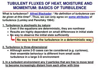
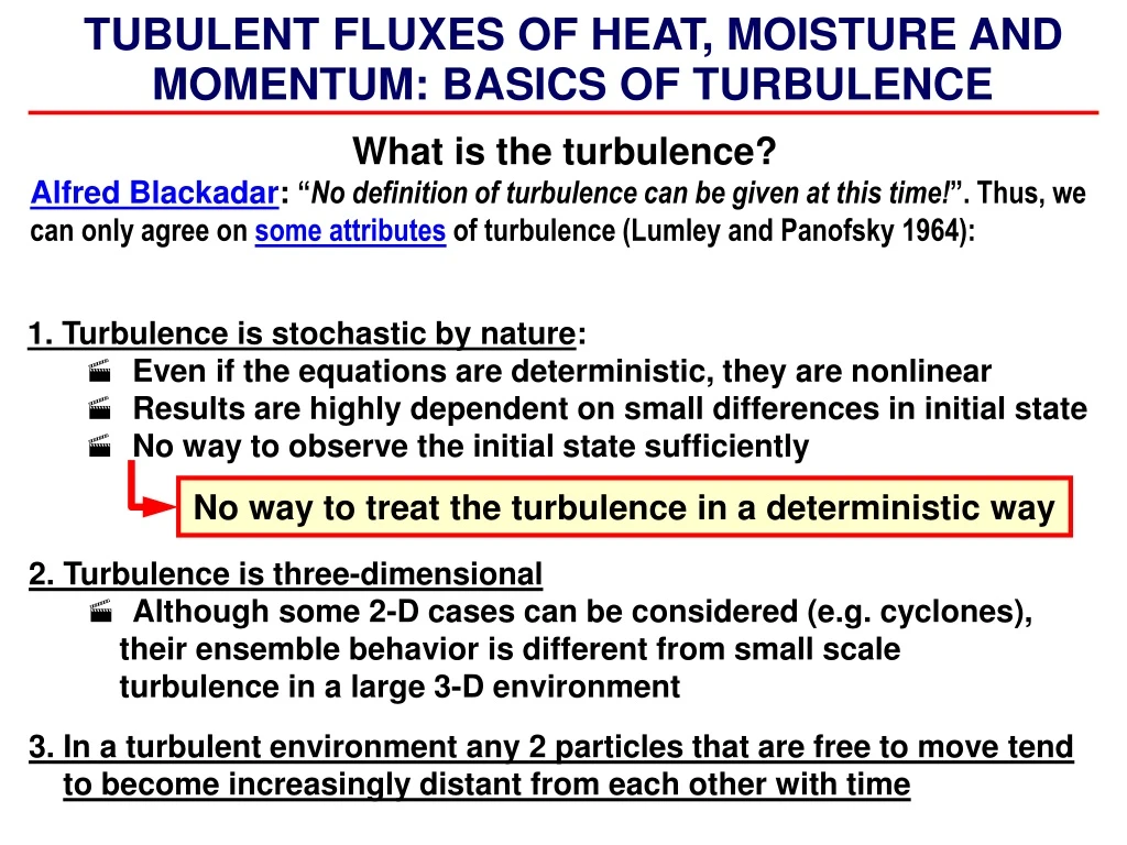
TUBULENT FLUXES OF HEAT, MOISTURE AND MOMENTUM: BASICS OF TURBULENCE What is the turbulence? Alfred Blackadar: “No definition of turbulence can be given at this time!”. Thus, we can only agree on some attributes of turbulence (Lumley and Panofsky 1964): 1. Turbulence is stochastic by nature: • Even if the equations are deterministic, they are nonlinear • Results are highly dependent on small differences in initial state • No way to observe the initial state sufficiently No way to treat the turbulence in a deterministic way 2. Turbulence is three-dimensional • Although some 2-D cases can be considered (e.g. cyclones), their ensemble behavior is different from small scale turbulence in a large 3-D environment 3. In a turbulent environment any 2 particles that are free to move tend to become increasingly distant from each other with time
Spectral energy Energy shift • 4. Turbulence is rotational by nature • Vorticity is an essential attribute of turbulence • 5. Turbulence is dissipative • The energy tends to shift from large-scale well organized eddies (small wave numbers) towards smaller eddies and, finally to molecular motions Vortices are stretched by turbulence, their diameter is reduced 6. Turbulence is a phenomenon of large Reynolds numbers • Large spatial dimensions • Small viscosity The space available for motions is LARGE in comparison to the dimensions of eddies
U L The Reynolds number Turbulent motions are highly dependent on the size of eddies and characteristic scales of the environment where the eddies exist. The Reynolds number is the ratio between the two lengths: Characteristic scale of the dimensions of the space available for all scales of motion Length which measures the thickness of the laminar (viscous) sub-layer (a layer where turbulence is not maintained due to its thickness), even if it is present in the other parts of the domain Lis defined by boundary configuration (e.g. depth of the channel, diameter of the pipeline). In the atmosphere gravity is essential, and turbulence is largely controlled by stable lapse rates. (laminar sublayer thickness) is related to viscosity: = / U (1) Where is kinematic viscosity, U is the velocity of the !LARGEST! scale of motions The dimensionless ratio between L and is the Reynolds number: Re = L/ = LU/ (2) In the pipes (pipelines): L usually is taken as a diameter, and mean current velocity stands for U Recr 1000
Osborne Reynolds's father was a priest in the Anglican church but he had an academic background having graduated from Cambridge in 1837, being elected to a fellowship at Queens' College, and being headmaster of first Belfast Collegiate School and then Dedham School in Essex. In fact it was a family with a tradition of the Church and three generations of Osborne's father's family had been the rector of Debach-with-Boulge. • Osborne was born in Belfast when his father was Principal of the Collegiate School there but began his schooling at Dedham when his father was headmaster of the school in that Essex town. After that he received private tutoring to complete his secondary education. He did not go straight to university after his secondary education, however, but rather he took an apprenticeship with the engineering firm of Edward Hayes in 1861. Reynolds wrote (actually in his application for the chair in Manchester in 1868) of his father's influence on him while he was growing up: • In my boyhood I had the advantage of the constant guidance of my father, also a lover of mechanics, and a man of no mean attainments in mathematics and its application to physics. • Reynolds, after gaining experience in the engineering firm, studied mathematics at Cambridge, graduating in 1867. As an undergraduate Reynolds had attended some of the same classes as Rayleigh who was one year ahead of him. As his father had before him, Reynolds was elected to a scholarship at Queens' College. He again took up a post with an engineering firm, this time the civil engineers John Lawson of London, spending a year as a practicing civil engineer. • In 1868 Reynolds became the first professor of engineering in Manchester (and the second in England). Kargon writes:- • ... a newly created professorship of engineering was advertised at Owens College, Manchester, at Ј500 per annum. Reynolds applied for the position and, despite his youth and inexperience, was awarded the post. • We should note in passing that Owens College would later become the University of Manchester. Reynolds held this post until he retired in 1905. His early work was on magnetism and electricity but he soon concentrated on hydraulics and hydrodynamics. He also worked on electromagnetic properties of the sun and of comets, and considered tidal motions in rivers. After 1873 Reynolds concentrated mainly on fluid dynamics and it was in this area that his contributions were of world leading importance. He studied the change in a flow along a pipe when it goes from laminar flow to turbulent flow. In 1886 he formulated a theory of lubrication.
Three years later he produced an important theoretical model for turbulent flow and it has become the standard mathematical framework used in the study of turbulence. • An account of Reynolds' work on hydrodynamic stability was published in 1883 and 1895]. The 1883 paper is called “An experimental investigation of the circumstances which determine whether the motion of water in parallel channels shall be direct or sinuous and of the law of resistance in parallel channels”. The 'Reynolds number' (as it is now called) used in modelling fluid flow which is named after him appears in this work. • Reynolds became a Fellow of the Royal Society in 1877 and, 11 years later, won their Royal Medal. In 1884 he was awarded an honorary degree by the University of Glasgow. By the beginning of the 1900s Reynolds health began to fail and he retired in 1905. Not only did he deteriorate physically but also mentally, which was sad to see in so brilliant a man who was hardly 60 years old. • Not only is Reynolds important in terms of his research, but he is also important for the applied mathematics course he set up at Manchester. Anderson writes in [3]:- • Reynolds was a scholarly man with high standards. Engineering education was new to English universities at that time, and Reynolds had definite ideas about its proper form. He believed that all engineering students, no matter what their speciality, should have a common background based in mathematics, physics, and particularly the fundamentals of classical mechanics. ... Despite his intense interest in education, he was not a great lecturer. His lectures were difficult to follow, and he frequently wandered among topics with little or no connection. • Lamb, who knew Reynolds well both as a man and as a fellow worker in fluid dynamics, wrote:- • The character of Reynolds was like his writings, strongly individual. He was conscious of the value of his work, but was content to leave it to the mature judgement of the scientific world. For advertisement he had no taste, and undue pretension on the part of others only elicited a tolerant smile. To his pupils he was most generous in the opportunities for valuable work which he put in their way, and in the share of cooperation. Somewhat reserved in serious or personal matters and occasionally combative and tenacious in debate, he was in the ordinary relations of life the most kindly and genial of companions.
Osborne Reynolds Born: 23 Aug 1842 in Belfast, IrelandDied: 21 Feb 1912 in Watchet, Somerset, England On the dynamical theory of incompressible viscous fluids and the determination of the criterion. Royal Society, Phil. Trans., 1895. Reynolds proceeded to measure the critical velocity for onset of eddies using three tubes of different diameter and in each case varying the water temperature. To a first approximation, the Reynolds Numbers based on these critical values of velocity were found to be the same (about 13000) for each of the tubes and for all water temperatures. He then set out to find the critical condition for an eddying flow to change into non-turbulent flow, referring to this as the `inferior limit'. To do this, he allowed water to flow in a disturbed state from the mains through a length of pipe and measured the pressure-drop over a five-foot distance near the outlet.
Reynolds’ three tubes Pressure measurements
The Reynolds approach to the equations of a turbulent fluid Reynolds separated each of the velocity components u, v and w into two parts: (3) Mean values Turbulent portion If we observe a sequence of velocities of particles at times that are sufficiently separated to be considered as uncorrelated with each other, the mean value of each sequence is independentof the other samples and themean values of deviations from the mean (u’, v’, w’) are zero: (4) Equation (4) represents the so-called ensemble averaging. Reynolds approach to the averaging of the equations of motion and the equation of continuity was to replace in each equation u, v and wby u, v and w+ u’, v’ and w’ u, v and w and to get the equations for the changes in
Continuity equation Lagrangian derivative The rate of change following the instantaneous motion Time and spatial derivatives at a fixed point Eulerian derivative Two forms of the continuity equation (5) (6)
(7) kstands for a dummy index which implies summation over the indices corresponding to the three Cartesian coordinate directions the derivative of product (8)
The Reynolds procedure(substituting from (3) and averaging the result)gives: (10) Averaging operators are applied to the derivatives, i.e.it is the derivative what is averaged ukuk - Reynolds postulates • Equation of continuity can be • applied to the mean motion and • mean velocity without change ! (11)
q Flux and general conservation equation Properties whose amounts are identified with a mass of fluid: • Specific humidity (the mass of water vapor per • unit mass of air) • Kinetic energy per unit mass • Specific entropy (Cpln) These properties are assumed to be conservative, i.e. they do not change just because of their motion Equation of the conservation of property q: (12) Source strength of the quantity q per unit mass Let’s assume that q is specific humidity. Then (12) can be expanded to
Let’s assume that q is specific humidity. Then (12) can be expanded to (13) Continuity equation multiplied by q term-by-term + (14) ? (15) The rate of convergence of a vector whose components are (ukq) The rate of change of the amount of q per unit volume measured at a fixed position The rate of internal production of qper unit volume at the same fixed point
xk V uk A A is a small area on the surface to one of the 3 axis. ukA is a volume of a cylinder with a height of uk(unit time). uk is the mass transported through a unit area of the surface to xk in one unit of time. ukq is the amount of property transported per unit area and per unit time across a surface to xk. This is flux of q in xk.direction Let’s average (15), substituting: q=q+q’, uk=uk+uk’: =0 (q+q’)(uk+uk’) = =quk+q’uk+quk’+q’uk’(16) The averaged conservation equation: (17) The flux due to mean state The eddy flux
Joseph Boussinesq (1842-1929) Ludwig Prandtl 1875-1953 Ernst Schmidt 1892-1975 The closure problem(K-theory) For q we use Taylor series expansion: We need to estimate the eddy flux of property q at ref. level zref (18) Parcel moves down through zref with a vertical velocity -|w’|. It has been last mixed with its environment at distance l1 from zref where it took its mean value. Deviation from the mean at reference level and the corresponding contribution to the flux: (19) Averaging over all parcels: Size of the largest energy containing eddy (mixing Prandtl length) (20) Kinematic exchange coefficients (eddy diffusivity)
3 components of the force x 3 surfaces = 9 stress components Stress is the tensor of rank 2 normal stresstangential stress Surface stress Stress is the force acting across the boundary surface and proportional to the area of surface, across which it acts. The sum of 3 diagonal components is a scalar invariant to any rotation of the axes. This sum is clearly related to pressure: When media is at rest the stress contains pressure only, when the media is a state of motion, the stress deviates from a simple pressure (while the pressure still remains the major component). The reminder is a viscous or tangential stress: symmetric tensor
Scalar product: displacement vector●tensor Scalar product: ½ displacement vector● Motion of the fluid, when velocity is expanded into Taylor series: Invariants of fluid motions: divergence + 1 missed ? To get the rate of pure deformation, we have to subtract out the divergence: Stress
total stress The motion equations General form of the Navier-Stokes equations (without Coriolis force): (21) Averaging: Molecular viscous stress Eddy turbulent stress (22) Molecular viscosity: ~10-5 m2s-1 Using K-theory: (23) Eddy diffusivity: ~1-10 m2s-1
Reynolds equations (averaged Navier-Stokes equations with Coriolis force): (24) Vertical momentum fluxes Conservation equations: Vertical fluxes of heat and moisture (25)
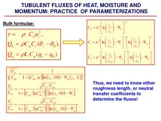
latent heat flux (evaporation) sensible heat flux momentum flux measurements parameterization