Download
1 / 35
380 likes | 654 Vues
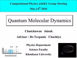
Computational Physics @KKU Group Meeting May,14 th 2010. Quantum Molecular Dynamics. Chutchawan Jaisuk. Advisor : Dr.Teepanis Chachiyo. Physics Department. Science Faculty. Khonkaen University. Outline. Introduction Part 1 (Simple masses and Spring) Part 2 (Central Force Motion)

E N D
ComputationalPhysics @KKU Group Meeting May,14th 2010 Quantum Molecular Dynamics Chutchawan Jaisuk Advisor : Dr.Teepanis Chachiyo Physics Department Science Faculty Khonkaen University
Outline • Introduction • Part 1 (Simple masses and Spring) • Part 2 (Central Force Motion) • Future work
Example 1) Simple Masses and Springs Analytical a) b) c) Simulation a) Basics Concept b) Computational Method c) Results and Discussion 1. Introductions Quantum + Molecular Dynamics
Example 2) Central Force Motion Analytical a) programming Simulation b) Results and Discussion
k m1 m2 x1(t) x2(t) x1* x2* m1 m1 q1(t) q2(t) Theory of motion (Analytical) แก้ปัญหาดังกล่าวด้วย “ Lagrange Mechanics ” โดยเลือก { q1,q2} เป็น generalize coordinate พิจารณาพลังงานรวมของระบบ กำหนดให้ m1 = m2 = m จากรูปข้างต้น นิยามให้ x1*, x2* คือ ตำแหน่งสมดุลของมวล x1(t) , x2(t) คือ ตำแหน่งของมวลแต่ละก้อน q1(t) , q2(t) คือ การกระจัดของมวลแต่ละก้อน
โดยมี และ เป็นผลเฉลย Lagrange Equation of Motion ได้ระบบของ differential equation คำนวณเทอมต่างๆ ดังนี้ สร้าง Lagrange Equation of Motion
ผลเฉลยของ Equation of motion ทดสอบผลเฉลยที่สมมุติขึ้นมา ______(1) จากสมการ (1) : ______(2) ______(3) สมมุติผลเฉลยของสมการการเคลื่อนที่ คือ จากสมการ (2) : ______(4) คำถาม : ผลเฉลยดังกล่าวทำให้สมการ (1) และ (2) เป็นจริงได้หรือไม่
ผลเฉลยของ Equation of motion สมการจะเป็นจริง ก็ต่อเมื่อ Determinant ของ matrix สัมประสิทธิ์ มีค่าเท่ากับศูนย์ จึงได้ว่า หรือ
k m k m m k m m m AnalyticalSolution a. ระบบสั่นได้เพียง ความถี่ค่าเดียว b. c. ระบบสั่นได้ 2 ความถี่
Simulation 1. Basic concept Use concept of 2nd Newton’s Law 1. กำหนด Initial position & velocity 2. คำนวณหาแรง (F) ที่กระทำต่อวัตถุ 3. คำนวณหาความเร็ว และ ตำแหน่ง เมื่อเวลาผ่านไป dt โดยอาศัยการทำซ้ำข้อ 2 และข้อ 3 เรื่อยๆ จะทำให้ทราบตำแหน่งวัตถุที่เวลาต่างๆ
X=0 X0 k m m 2. Computational Method 2. Set force function & simulate Use to simulate 1. Set parameters of system
k m 3. Result & Discussion a.)
k m m b.)
k m m m c.) กราฟเริ่มจะซับซ้อนขึ้นมากกว่า 2 ตัวอย่างที่ผ่านมา
Case a.) & b.) Time Domain หาได้จากการพิจารณากราฟ Fourier Transform ถาม : มีวิธีอื่น ที่จะหาค่าความถี่ ได้อย่างแม่นยำหรือไม่ ? Frequency Domain ตอบ: Fourier Transform
Fourier transform ระบบสั่นด้วย 2 ความถี่ คือประกอบด้วย f1 = 0.107 Hz และ f2 = 0.195 Hz
simulation f2_sim = 0.195 Hz f1_sim = 0.107 Hz Analytical Comparison between simulation & analytical จากทั้งหมดที่ผ่านมา สรุปได้ว่า ผลจาก Simulation มีความสอดคล้องกับผลเชิง Analytical
Function 1 Loop 2 3 4. C-programming Mathcad C-programming Skill Structureprogramming Function Array
จากที่ได้เรียนรู้กลไกทาง C-programming ในการเขียน simulation program ก็นับเป็นจุดเริ่มต้น เพื่อพัฒนาการวิเคราะห์การเคลื่อนที่จาก 1D ไปยัง 3D
z y z x y x Theory of motion 1. center of mass 2. reduce mass กรณี 2 อนุภาค การเคลื่อนที่นั้นควรจะให้จุด CM เป็นจุดกำเนิดของกรอบอ้างอิง ทบทวนพื้นฐานเหล่านี้ได้จาก Classical dynamics of particles and systems(Chapter 9)
z y x 3.Equation of motion โดยอาศัย Lagrange equation จะสามารถหาสมการการเคลื่อนที่ได้ซึ่งเขียนได้เป็น
3. If is the planet’s semi-major axis (one-half the ellipse’s greatest width) , then where Tis the planet’s period. 4. Kepler’s Law 1 . All planets move in ellipses, with the sun at one focus. 2. A line from the sun to the planet sweeps out equal area in equal times.
Simulation Use concept of 2nd Newton’s Law Force form
2 3 4 5 6
z y x 2.Result and Discussion Condition for all case study of simulation 1.) Set : m1 = 10,000 kg, m2 = 1kg 2.) Assume : G = 10 N m2 / kg2 A.)
y z x B.)
Table-1 Relation betweena (semi-major axis) andT (period) Plot graphand Analyse
Analytical : Simulation : Comparisonsimulation & Analytical The result from simulationis consistent with analytic.
Future work • Dynamics of Chemical Reactions • Rovibrational Motions of Molecules • Molecular Reactions on Surfaces • Molecular Reactive Scattering Process • etc.