Download
1 / 37
370 likes | 487 Vues
Development of a Statistical Dynamic Radiation Belt Model. S. Benck, L. Mazzino, V. Pierrard, M. Cyamukungu, J. Cabrera. benck@spaceradiations.be Center for Space Radiations (CSR) UCL, Louvain-La-Neuve, Belgium. ESWW5, Brussels, Belgium, 17-21 November 2008. Introduction. Steady state.

E N D
Development of a Statistical Dynamic Radiation Belt Model S. Benck, L. Mazzino, V. Pierrard, M. Cyamukungu, J. Cabrera benck@spaceradiations.be Center for Space Radiations (CSR) UCL, Louvain-La-Neuve, Belgium ESWW5, Brussels, Belgium, 17-21 November 2008
Introduction Steady state GS pobabilities Flux variations Decay times Conclusion McIlwain in 1966 identifies 5 « Processes acting upon outer zone electrons » Process 1: Rapid non adiabatic acceleration Process 2: Persistent decay Process 3: Radial Diffusion Process 4: Adiabatic Acceleration Process 5: Rapid Loss Measured radiation dose (black) compared to the static model prediction (red) based on flux averages (see Glossy brochure of the SREM from Contraves-PSI) (From McIlwain, 1996 AGU)
Introduction Steady state GS pobabilities Flux variations Decay times Conclusion . . . flux = steady state background + geomagnetic activity dependent value T fst= Steady state flux measured fn = The expected flux variation following a storm (average) Dfres= Diff. between. flux before storm and steady state flux T= Decay time of flux for a given position and energy d = Time elapsed from the storm min. Dst_prev (or drop- out min) tof0 (Maximum flux) N = Number of bins in Dst range S = Solar par. that indicates phase within the solar cycle Type = Type of storm: CME, CIR, Mix F(Dst_prev) = Flux var. induced by prev. storm of min Dstprev Dst prev = The min. value reached by Dst in the prev. storm L. Mazzino, et al (2008)
Introduction Steady state GS pobabilities Flux variations Decay times Conclusion ~100 days fst
Introduction Steady state GS pobabilities Flux variations Decay times Conclusion Fst as a function of longitude, latitude and altitude Fst as a function of L (B>0.3 G)
Introduction GS probabilities Steady state Flux variations Decay times Conclusion 50 years of Dst and sunspot number data, including ~1200 storms have been analyzed Black dots correspond to Dst minimum of the GS. The number of storms is outlined for each of the solar cycles (orange). Solar maximum and minimum activity are delineated (green and blue lines respectively, dates indicated), corresponding to solar cycles 19 (incomplete), 20, 21, 22 and 23. Sunspot number is plotted on the black curve with superimposed smoothed curve in red.
Introduction Steady state GS pobabilities Flux variations Decay times Conclusion • Probability of two successive GS with a given time interval, for the declining phase of the different solar cycles Poisson distribution • Probability of having a GS of a given Dstk after a previous GS of any magnitude, for the declining phase . • Nice agreement with: Tsubouchi and Omura, Long-term occurrence probabilities of intense geomagnetic storm events, Space Weather, 2007
Introduction Flux variations Steady state GS pobabilities Decay times Conclusion DF and d as a function of GS type Electron fluxes data: Two LEO Satellites, Ee= 200 keV – 1.2 MeV DEMETER/IDP SAC-C/ICARE Orbit at 710 km 98.23 deg. Incl. Orbit at 702 km 98.2 deg. Incl. (Picture: Courtesy of CONAE) http://www.conae.gov.ar/sac-c/ (Picture: Courtesy of CNES) http://smsc.cnes.fr/DEMETER/
Introduction Steady state GS pobabilities Flux variations Decay times Conclusion • Flux enhancement (DF) and Time interval between storm and flux max ()
Introduction Steady state GS pobabilities Flux variations Decay times Conclusion • Storm type definition TYPE 1 (mainly CME) TYPE 2 (mainly CIR) short DBz/Dt, ’’peak’’, Dt ~3-4h long DBz/Dt, ’’inconsistent’’, Dt >7h • Kataoka and Miyoshi, “Flux enhancement of radiation belt electrons during geomagnetic storms driven by coronal mass ejections and corotating interaction regions.” Space weather, 2006
Introduction Steady state GS pobabilities Flux variations Decay times Conclusion • The time interval between magnetic storm and flux maximum (d) seems to be linear for the classified isolated storms, but random for all other storms. Need more parameters TYPE 1(yellow), TYPE 2 (red)
Introduction Steady state GS pobabilities Flux variations Decay times Conclusion • Resultant flux enhancement DF as a function of storm severity, corresponding to isolated TYPE 1 (yellow), TYPE 2 (red), and mixed non isolated storms (blue)
Introduction Steady state GS pobabilities Flux variations Decay times Conclusion slope L-parameter slope TYPE 2 • For all L values, the flux enhancement increases steeper with Dstmin (slope > 0) for lower energies • For all energies the slope decreases with L TYPE 1 • At low L the flux enhancement increases steeper with Dstmin (slope > 0) for lower energies • At high L the flux enhancement decreases steeper with Dstmin (slope < 0) for lower energies. L-parameter
Introduction Decay times Steady state GS pobabilities Flux variations Conclusion • Decay time constant (loss timescales) of electron fluxes (T) DEMETER/IDP – SACC/ICARE comparison • Condition of measurement: • The time resolution is 12 h • The maximum flux after storm must occur 3 days before the defined end of the storm
Introduction Steady state GS pobabilities Flux variations Decay times Conclusion • Decay time of electron fluxes (T) as a function of position and energy A pattern that is often observed during individual storms: At low L, the decay time decreases with increasing energy, while at high L this pattern is inversed. • Meredith et al, “Energetic outer zone electron loss timescales during low geomagnetic activity.” JGR (2006) 3<L<5, T(Ehigh) > T (Elow), for l<15° • Lyons et al, “Pitch-angle diffusion of radiation belt electrons within the plasmasphere.” JGR (1972) T=min at around L =3Re (theory)
Introduction Steady state GS pobabilities Flux variations Decay times Conclusion • Cases where the electron flux increases continuously (Benck et al, Study of correlations between waves and particle fluxes measured on board the DEMETER satellite, Advances in Space research (2008) • Meredith et al, “Evidence for acceleration of outer zone electrons to relativistic energies by whistler mode chorus.” Annales Geophysicae (2002) d (wave activity) ?
Introduction Conclusion Steady state GS pobabilities Flux variations Decay times • Identified Parameters • Steady state Fst • Storm occurence and related probabilities • Dstprev, Dstk (1224 storms!) • t (time interval between two storms) • Solar Cycle parameter (SSN) • Flux variations during storm time • Type of storm (presently 2 types) • d (elapsed time between storm max (Dstmin) and maximum flux) • Maximum Flux and Flux enhancement DF • T (Decay time) • L. Mazzino et al, Development of a statistical dynamic radiation belt model: Analysis of storm time particle flux variations, ESA Ionizing Radiation Detection and Data Exploitation Workshop proceedings, 2008 • Solar parameters data: Courtesy of GSFC Space Physics Data Facility http://omniweb.gsfc.nasa.gov/index.html • SAMPEX DATA: Courtesy of SAMPEX Data Center http://www.srl.caltech.edu/sampex/DataCenter/ • SAC-C Data: Courtesy of CNES/DCT/AQ/EC Section, ONERA/DESP and CONAE • Sunspot Number Data: Courtesy of Solar Influences Data Analysis Center – SIDC, Belgium
Example of geomagnetic storm Storm Sudden commencement Recovery phase Main phase Strength of storm: Minimum Dst reached
Introduction Steady state GS pobabilities Flux variations Decay times Conclusion • steady state background i.e. mapping of quiet time fluxes + • Geomagnetic storm (GS) prediction (Dst<-50 nT) - Occurrence probability • Flux variation associated to GS, as a function of energy, position and type of storm • Flux decay time as a function of energy, position, ... Statistical dynamic radiation belt model • L. Mazzino et al, Development of a statistical dynamic radiation belt model: Analysis of storm time particle flux variations, ESA Ionizing Radiation Detection and Data Exploitation Workshop proceedings, 2008
Dst Butterworth filter: z = cutoff frequency Dst data (black) withfiltered data (red): The second graph shows the filter detail, and the fourth shows a closed up of the event, with actual amplitude of the storm in green. (Dst Data: Courtesy of World Data Center for Geomagnetism, Kyoto)
Introduction Steady state GS pobabilities Flux variations Decay times Conclusion Sunspot Number Maxima (smoothed) Solar cycle #20: 109 Solar Cycle #21: 159 Solar Cycle #22: 157 Solar Cycle #23: 121 • Correlation between number of storms per month for different phases in a solar cycle with the Sunspot Maximum corresponding to that cycle.
Introduction Steady state GS pobabilities Flux variations Decay times Conclusion • Probability of having a storm with intensity Dstk considering that the previous one was of intensity Dstprev All Dstmin given in absolute value Histogram of Dstk vs. Dstprev number of bins = 100
Introduction Steady state GS pobabilities Flux variations Decay times Conclusion • Probability of having a storm with intensity Dstk considering a given time interval elapsed since the previous storm All Dstmin given in absolute value For few events the time interval between storms is greater than 100 days, and the time interval between those storms can be used to find the steady state. • Nice agreement with: Tsubouchi and Omura, Long-term occurrence probabilities of intense geomagnetic storm events, Space Weather, 2007 Histogram of Dstk vs. time interval, number of bins = 100
Introduction Steady state GS pobabilities Flux variations Decay times Conclusion • Sunspot number maximum is a good parameter to represent solar cycle activity vs. total number of storms. Solar Parameter (S): Sun Spot Number Sunspot Number Maxima (smoothed) Solar cycle #20: 109 Solar Cycle #21: 159 Solar Cycle #22: 157 Solar Cycle #23: 121 The total number of storms per month in a cycle correlates directly to the severity of the solar cycle: For solar cycles with higher SSN maxima, SC 21 and SC 22,the total number of storms is higher than for SC 20 and SC 23 with lower maxima
Introduction Steady state GS pobabilities Flux variations Decay times Conclusion The distribution of time interval between storms for all 1204 storms in the last 50 years seems to be Poisson-distributed. Histogram of smoothed Sunspot number vs. Time interval between storms (number of bins = 25 time resolution = 10 days) • Probability of having a certain time interval between storms considering the sunspot number
Difference of time interval distribution function depending on phase and severity of solar cycle activity 27
Geomagnetic storm: particle flux enhancement • Fluxes DEMETER
(SAC-C Data: Courtesy of CNES/DCT/AQ/EC Section, ONERA/DESP and CONAE)
Results: Fluxes Resultant maximum flux as a function of storm severity, corresponding to isolated CME’s (yellow), CIR’s (red), and mixed non isolated storms (blue) Resultant flux enhancement difference as a function of storm severity, corresponding to isolated CME’s (yellow), CIR’s (red), and mixed non isolated storms (blue)
TYPE 1(yellow), TYPE 2 (red) (SAC-C Data: Courtesy of CNES/DCT/AQ/EC Section, ONERA/DESP and CONAE)
TYPE 2 33
Introduction Steady state GS pobabilities Flux variations Decay times Conclusion • Decay time of electron fluxes (T) independent of Dst
We need a reference invariable with time • Magnetic Coordinates: McIlwain (1961-1966) Hess (1968) • In a dipole: Illustration from: http://en.wikipedia.org/wiki/L-shell
CIR’s: Corotating Interaction Regions Akasofu and Hakamada, 1983 Hundhausen, 1972 MHD simulation of (1) high speed streams which cause the development of CIR structure and (2) the propagation of transient shocks which also modify the CIR structure (bottom two panels particularly) Schematic illustration of a fast stream interacting with a slow stream
CME’s: Coronal Mass Ejection Cravens, 1997 Space Weather Laboratory, George Madison University Schematic of a coronal mass ejection in the form of a magnetic cloud with a shock.


![[The Virtual Radiation Belt Observatory]](https://cdn2.slideserve.com/5073406/the-virtual-radiation-belt-observatory-dt.jpg)