Download
1 / 23
230 likes | 414 Vues
Control of a Solution Copolymerization Reactor using Piecewise Linear Models. Leyla Özkan APACT-03 York, UK April 30 th , 2003. Presentation Outline. Motivation Multi-Model Predictive Control Formulation Implementation on MMVA Solution Co-polymerization Reactor Stability Analysis

E N D
Control of a Solution Copolymerization Reactor using Piecewise Linear Models Leyla Özkan APACT-03 York, UK April 30th , 2003
Presentation Outline • Motivation • Multi-Model Predictive Control Formulation • Implementation on MMVA Solution Co-polymerization Reactor • Stability Analysis • Conclusion APACT03-30 April, 2003
Motivation • Polymerization reactors • Complex nonlinear kinetics and behavior • Difficult to specify control objectives • Global competition • Strict requirements on polymer properties • Grade transitions common • Control objective • Minimize grade transition time Reduce Off-Specification Product APACT03-30 April, 2003
min J ( k ) p u ( . ) Past Future Set point dx Predicted y = f ( x , u , t ) dt Closed loop y Open loop u £ £ u u u min max £ £ y y y min max Closed loop u k k+1 k+Hc k+Hp Hc Hp Model Predictive Control • Model Predictive Control • Class of control algorithms that solves optimization problem at every instant APACT03-30 April, 2003
[ ] ¥ T = + + + J x ( k m | k ) Q x u Ru ( k m | k ) å ¥ I T + + ( k ) ( k m | k ) ( k m | k ) finite horizon cost infinite horizon cost m = 0 2 å + + x ( k m | k ) 2 n + + + + u u ( ( k k m m | | k k ) ) x ( k m | k ) R Q 2 2 = m n+1 I å + Q R I = m 0 • Effective in terminal region • Bounded by • State feedback controllaw T + + + + x ) ) ( k n 1 P x ( k n 1 Multi-Model Predictive Control • Infinite horizon objective function • Free input variables • Forces states towards • terminal region APACT03-30 April, 2003
x(k+1|k), u(k+1|k) x(k+2|k), u(k+2|k) x(k|k), u(k|k) n+1 m (x,u) = (0,0) u(k+m|k)=Kx(k+m|k) Terminal region x(k+n+1|k) Quasi-infinite horizon strategy APACT03-30 April, 2003
Define sequence of regions and models t J J ¥ n OP2 x2 OP1 x1 Illustration of multi-model predictivecontrol Control Recipe If x terminal region quasi-infinite horizon If x terminal region infinite horizon APACT03-30 April, 2003
g min é ù 1 * * * * * L ê ú 0 . 5 g Q x ( k | k ) I 0 0 0 0 0 I ê ú 0 . 5 ê ú g R u ( k | k ) 0 I 0 0 0 0 ê ú 0 . 5 ³ + g 0 Q x ( k 1 | k ) 0 0 I 0 0 0 ê ú I 0 . 5 ê ú + g R u ( k 1 | k ) 0 0 0 I 0 0 ê ú M O ê ú ê ú + + x ( k n 1 | k ) 0 0 0 0 0 Q ë û é ù T 0 . 5 T 0 . 5 T + Q ( A Q B Y ) QE QQ Y R t t t t I t ê ú T T + + x x ( A Q B Y ) Q b b b e 0 0 ê ú t t t t t t t ê ú T T ³ 0 x - x - E Q e b ( I e e ) 0 0 t t t t t ê ú 0 . 5 ê ú g Q Q 0 0 I 0 I ê ú 0 . 5 g R Y 0 0 0 I ë û t The resulting LMI problem Finite horizon x(k) terminal region Infinite horizon APACT03-30 April, 2003
g min x Q , , Y i s.t. é ù T 1 x ( k | k ) ³ 0 ê ú ê ú x ( k | k ) Q û ë and é ù T 0 . 5 T 0 . 5 T + Q ( A Q B Y ) QE QQ Y R i i i i I i ê ú T T + + x x ( A Q B Y ) Q b b b e 0 0 ê ú i i i i i i i ê ú T T ³ 0 x - x - E Q e b ( I e e ) 0 0 i i i i i ê ú 0 . 5 ê ú g Q Q 0 0 I 0 I ê ú 0 . 5 g R Y 0 0 0 I ë û i - - - 1 1 1 = g x = l = P Q K Y Q i i Özkan, L. et.al. , Control of a solution copolymerization reactor using multi-model predictive control, Chem. E. Science, 58:1207-1221, 2003 The resulting LMI problem Feasible ONLY IF bi=0 (x(k) terminal region) APACT03-30 April, 2003
Consider j = 1 , 2 , … , n £ u ( k ) u u k 0 j j , max ³ Finite horizon cost: Infinite horizon cost: Impose directly ( u ( k + m | k ) k + m | k ) = Kt x + £ Exists s.t. X u ( k m | k ) é ù X Y j 2 t ³ £ 0 X u ê ú jj j , max u Y Q ë û j t , max m = 0 , 1, …, n j j = = 1 1 , , 2 2 , , … … , , n n u u m = n+1 ,…, Input Constraints APACT03-30 April, 2003
Monomer (FA) Monomer (FB) Initiator (FI) Coolant Solvent (FS) Coolant Transfer Agent (FC) Polymer Solvent Unreacted feed Inhibitor (FZ) Richards, J. R. et.al. , Feedforward and Feedback Control of a Solution Co-polymerization Reactor, AIChE Journal, 35(6):891-907, 1989 MMVA Solution Copolymerization Reactor • Characteristics: • Based on free radical mechanism • Realistic industrially • 12 states, 4 outputs • Dynamics depends on monomers’ feed ratio Challenge: Optimization problem involves 200–300 variables APACT03-30 April, 2003
Step input (FA/FB: 0.2 0.25) 4 OP 2 3.8 Mw/E4 (kg/kmol) 3.6 OP 1 3.4 0 10 20 30 40 50 time (h) Implementation on MMVA copolymerization reactor • Manipulated variables • FA, FB, FC, Tj • Obtaining multiple models • Select new desired operating point • Assume a trajectory APACT03-30 April, 2003
(x,u) - (0,0) • Desired operating point • Driving force • Linear models are updated accordingly • Norm measure to define sequence of linear models x3 x x(k|k) x2 x1 t Implementation on MMVA (cont’d) • Simplifications • Only terminal region approximated as ellipsoid APACT03-30 April, 2003
Ap Y 30 30 0 0 10 10 20 20 time (h) time (h) Implementation on MMVA (cont’d) • Effect of number of linear models 2 models 4 353.5 3 models 353.4 3.8 T (K) 353.3 4 models Mw/E4 (kg/kmol) 353.2 3.6 353.1 3.4 Off–spec. (kg) 0.64 27 26 0.62 Open loop 302.4 25 0.6 2 models 134.8 Gpi (kg/h) 0.58 24 3 models 110.1 23 0.56 4 models 109.8 0.54 22 APACT03-30 April, 2003
MPC • Lyapunov Approach • dx(t)/dt=f(x) and x=0 equilibrium • V(x) • V(x)>0, x 0 and V(x)=0 x=0 • d V/dt<0, x 0 Asymptotically stable origin V(x) Time Stability Analysis • Conventional control • Check eigenvalues of closed-loop system APACT03-30 April, 2003
Discrete components Continuous dynamical systems Logic commands (switches,automata) Hybrid systems Hybrid systems • Definition: • Dynamical systems with continuous and discrete state variables APACT03-30 April, 2003
Branicky, M.S., Multiple Lyapunov functions and other analysis tools for switched and hybrid systems, IEEE Trans. Automatic Control, 43(4):475-482, 1998. Multiple Lyapunov Functions • Consider Vi :i=1,2,…,N • Given S={x0: (i0,t0),(i1,t1),…,(iN,tN),..} • Denote • T: increasing sequence of times t0,t1,…tN • (T):even sequence of T:t0,t2,t4, If Viis monotonically non-increasing on(T) then system is stable in the sense of Lyapunov APACT03-30 April, 2003
Interpretation for N=2 V1(x) t0 t1 t2 t3 t4 t5 t6 V2(x) Multiple Lyapunov Functions • Easy to interpret • N candidate Lyapunov functions • Requires stable subsystems APACT03-30 April, 2003
Theorem Ifx(k) terminal region, the quasi–infinite horizon optimization problem is solvedincluding the contractive constraint. If x(k) terminal regionthe infinite horizon optimization problem is solved. The closed loop system is stable if the feasible solutions of the control strategy defined are implemented in a receding horizon fashion Multi-Model Predictive Control with Stability Guarantee • Contractive constraint • (k) < (k-1) x terminal region • Stability Analysis APACT03-30 April, 2003
Proof • Candidate Lyapunov function terminal region Ï g ì ( k ) x ( k ) = V í a ( ( x )) T terminal region Î x ( k ) Px ( k ) x ( k ) î Multi-Model Predictive Control with Stability Guarantee • Remarks • Stability results depend on feasibility • States are measurable • @ k=ts • V(x(ts))-V(x(ts-1))<0; not required APACT03-30 April, 2003
1 10 0 10 (k) xT(k)Px(k) -1 10 log (V) -2 10 -3 10 -4 10 0 5 10 15 t(h) MMVA solution copolymerization revisited • Observations • V monotonically decreasing • ts=7.0 and 7.75 h APACT03-30 April, 2003
Summary and Conclusion • Multi-model control algorithm is developed • Hybrid structure • Implemented on a high dimensional problem • The effect of number of linear models • Decrease in transition time • Computational difficulty • Number of free input variables • Large size LMI’s solved on a realistic problem • Stability analysis • Contractive constraint • Multiple Lyapunov Functions APACT03-30 April, 2003
Thank you for your attention Leyla Özkan APACT03-30 April, 2003