Download
1 / 23
230 likes | 366 Vues
Observational Consequences of Inhomogeneous Cosmology. John W. Moffat, Perimeter Institute for Theoretical Physics. Talk given at the Albert Einstein Century Conference, UNESCO Building, Paris, July 21, 2005.

E N D
Observational Consequences of Inhomogeneous Cosmology John W. Moffat, Perimeter Institute for Theoretical Physics Talk given at the Albert Einstein Century Conference, UNESCO Building, Paris, July 21, 2005 astro-ph/0504004 astro-ph/0505326 hep-th/0507020
Contents 1. Introduction 2. Exact Inhomogeneous spherically symmetric solution 3. Cosmic variance and observer, location dependence of physical quantities 4. Non-Gaussian distribution of CMB fluctuations and alignment of lower l multipoles 5. Can a late-time inhomogeneous density enhancement (void) describe an accelerating universe? 6. Conclusions
1. Introduction • The standard FLRW cosmology can be considered as a first approximation to a description of the large scale structure of the universe. It provides a simple and successful description of the CMB and the expansion of the universe. However, the model can fail to describe important features of the data such as an uneven distribution of fluctuations that have been claimed to exist in the WMAP data, the possible anomalous alignment of lower l multipoles in the WMAP sky data and potential claims of non-gaussian behaviour. • Such effects can be due to anisotropic and inhomogeneous distributions of matter. Calculations have been performed of perturbations of the smooth FLRW background spacetime. These perturbation calculations fail in the non-linear inhomogeneous region associated with large scale structure. We must therefore consider non-perturbative solutions.
Claims have been made that sub-horizon and superhorizon modes that are created by inflation can lead to a negative deceleration parameter q through second order perturbations on a FLRW background spacetime (Kolb, Matarrese, Riotto… others). These claims cannot at present be substantiated due to the failure of the perturbation theory at late times. • It is possible that an exact inhomogengeous description of the late-time non-linear regime associated with galaxies, clusters of galaxies and voids could lead to a negative q and describe the accelerating expansion of the universe without a negative pressure dark energy or a cosmological constant Lambda. We shall investigate these claims in the following using the Raychoudhuri equation and a spatial volume averaging of scalar physical quantities such as the time evolution of the expansion parameter theta and the average deceleration parameter <q>. • A late-time inhomogeneneous model will lead to a cosmic variance in cosmological observables such as luminosity distance and deceleration parameter, due to the observer location dependence of measurements.
2. Exact Spherically Inhomogeneous Symmetric Solution • Consider the spherically symmetric inhomogeneous line element: The inhomogeneous Friedmann equations take the form (JWM, 2005): f(r) is an arbitrary function of r, rho=rho(r,t), p=p(r,t) and Lambda is the cosmological constant.
A late-time inhomogeneous open solution metric describing an under-dense void is given by • A parametric solution is for f^2=1 + r^2 is obtained in the Lemaitre-Tolman-Bondi (LTB) matter dominated solution:
f(r) and beta(r) are arbitrary functions of r. The beta(r) can be be specified on some hyper-surface t=t_0. The metric is singular for u=0 and R(r,t)=0. The singular surface can describe the surface of last scattering when the solution is matter dominated with zero pressure. The hyperbolic FLRW model is obtained for This leads to the FLRW metric solution
We choose the change of radial coordinate We postulate that beta(r) approaches a maximum value at the end of galaxy and cluster formation with the model: where a, b and alpha are positive constants, beta(0)=0 and beta(r*) a for r* >> b. The metric for f(r*) 1 becomes the flat space FLRW Einstein de Sitter metric
We have We obtain for beta(r*) 0 the homogeneous and isotropic flat space Einstein-de Sitter solution which describes the matter dominated epoch near the surface of last scattering with small anisotropy contrast ~ 10^(-5) corresponding to the WMAP data 20 < z < 10^3. The metric is
3. Cosmic variance and observer, location dependence of physical quantities • The luminosity distance between an observer at the origin of the coordinate system t_0 and the source at t_e, r_e, theta_e, phi_e is The red shift considered as a function of r along the light cone is We have defined the angular Hubble parameter and the radial parameter that replaces
For the late-time late dominated era, we define the deceleration parameter: We obtain for our open hyperbolic, under-dense void solution The variance of q is given by the exact expression
We find that different observers located in different causally disconnected parts of the sky will observe different values for the luminosity distance d_L(r,t), the red shift z(r,t) and the deceleration parameter q(r,t). This can lead to a cosmic variance and an intrinsic observational uncertainty in these physical quantities. 4. Non-Gaussian distribution of CMB fluctuations and alignment of lower l multipoles In the LTB solution for p=lambda=0, the growth of the angular power spectrum is given by • We see that the observed CMB temperature fluctuations will differ in different parts of the sky, depending on the value of r and the location of the observer. In the global FLRW model the observed CMC is the same in all directions in the sky.
There are preliminary indications for a non-zero difference in the power spectrum extracted from WMAP data in the northern and southern hemispheres oriented along the galactic co-latitude and longitude (80^0, 57^0), close to the ecliptic pole for l ~ 2 – 40 (Hansen, Banday and Gorski, 2004; Eriksen et al. 2004). This could indicate a non-Gaussianity in the WMAP data (Coles et al., Cruz et al., Land and Maguiejo; Oliveira et al.; Spergel and Wandelt, 2003, 2004). From the LTB model we find due to a difference in t_(LTB)(r) in the locations of the northern and southern hemispheres (JWM, 2005): where t_(Sigma) denotes the singular surface of last scattering. • The apparent temperature and red shift as observed in the direction theta is
The dipole, quadrupole and octopole moments, are • An observer looking toward the center of the spherically symmetric LTB density enhancement will see an axially symmetric distribution. The dipole, quadrupole and octopole moments will be aligned in this plane, with the angle theta defining the trajectory of a light ray arriving to the observer located as (t_0, r_0). The dipole contribution is small and undetected in the WMAP data, while there are indications that the quadrupole and octopole moments are aligned to a statistically anomalous degree (de Oliveira-Costa et. 2003; Tegmark et al. 2003; Starkman et al. 2003; Schwarz et al. 2003; Katz and Weeks, 2004; Ralston and Jain, 2004). • There have been indications of anomalously low l values in the WMAP power spectrum.
5. Can a late-time inhomogeneous density enhancement (void) describe an accelerating universe? • Let us set the cosmological constant lambda=0. WE obtain for the LTB under-dense inhomogeneous solution: If we have then q can be negative and perhaps cause the universe to accelerate with Lambda=0 and no dark energy.
We shall now show that for the LTB model the Raychoudhouri equation leads to a negative conclusion. Consider a time-like vector : with and The vorticity tensor is given by where and the shear tensor • The volume expansion is given by and the Raychoudhuri equation reads for geodesic world lines From Einstein field equations we have for p=Lambda=0:
For our under-dense void solution The LTB model uses synchronous comoving coordinates g_(00)=1 and V^0=1, V^I=0 (I=1,2,3) and • We might conclude that if then q can be negative leading to a local acceleration of the universe. However, in our synchronous comoving coordinates, the vorticity is zero From late-time observations we expect for vorticity Omega_(omega)~ 10^(-5).
Recent attempts to explain dark energy focus on “back-reaction” effects of inhomogeneities at late-times with Lambda=0. This will solve the “coincidence” problem, because the galaxy inhomogeneities occur lately in the non-linear regime evolution of the universe, 0 < z < 20, and supernovae measurements are made for 0.4 < z < 1.7 (Perlmutter, Riess 1999-2004). • We define a spatial averaging (Ellis, 1984; Kolb, Matarrese, Riotto, 2005; Buchert, 2005 for a scalar field : • The volume averaging does not commute with its time evolution For the spatially averaged expansion theta: Inserting Raychoudhuri’s d/dt(theta), we get for the spatially averaged scale factor in a FLRW background spacetime:
We have the first integral for our irrotational FLRW background spacetime (Buchert, 2005): The back-reaction source term is If the condition is satisfied • Then we have a local accelerating path of the universe. Whether this condition can be observationally satisfied is still a matter of controversy. • Note that in the late-time non-linear regime the perturbation theory fails. We should now return to the exact inhomogeneous model.
We can now apply the same spatial averaging to a scalar in the inhomogeneous model (JWM, 2005): We can define an effective scale factor . The volume average of the scalar does not commute with its time evolution: • For the average expansion theta(r,t), we can obtain the expression: . Substituting the Raychoudhuri equation for Lambda=0 and zero vorticity omega=0, we get
If we can satisfy the condition where P_D is a function of the shear sigma and the expansion parameter theta, then the averaged deceleration parameter can be negative, • corresponding to an acceleration of a local observed region of the universe, even though the vorticity is zero in our synchronous comoving gauge. • We can apply this result to our LTB exact open, void solution in the non-perturbative late-time regime and obtain an accelerating expansion in our observable region of the universe without negative pressure fluids or a cosmological constant. It would also resolve the “coincidence problem”. 6. Conclusions • An exact solution is obtained from Einstein’s gravitational field equations which describes the universe from the inhomogeneous and isotropic FLRW near the surface of last scattering to the late-time, non-linear regime describing large scale structure.
The preliminary anomalies that have been observed in the WMAP data, such as the possible alignment of lower l multipoles along the “axis of evil” and the uneven non-Gaussian distribution of fluctuations in the northern and southern hemispheres, can be explained from the late-time inhomogeneous, spherically symmetric LTB model due to the location dependence of the off-center observer. • By introducing a required spatial volume averaging procedure for scalar physical quantities, the averaged scalar expansion parameter theta in the Raychoudhuri equation and its averaged time evolution can lead to a negative deceleration parameter <q>. This allows for an accelerating expansion in our local observed region of the universe without negative pressure dark energy or a cosmological constant. The “coincidence problem” as to why the acceleration of the expansion started “now” is resolved, since the large scale structure associated with galaxies, clusters of galaxies and voids occurred for red shifts 0 < z < 10-20, which includes the observed “dimming” of the supernovae at 0.4 < z < 1.7
Why is the cosmological constant zero (or very small)? If we attribute the accelerating expansion of the universe to gravitational effects of late-time inhomogeneity, then we still have to explain why Lambda=0! • I believe the solution to the CCP lies in reinterpreting the nature of the vacuum state in quantum field theory and quantum gravity (JWM, 2005). This requires a revision of quantum field theory including gravity, taking account of positive and negative energy fermions and bosons by introducing an indefinite metric in Hilbert space, and using Dirac’s idea of a completely filled negative energy sea of fermions and bosons. To stabilize the boson vacuum, we postulate that negative energy bosons satisfy a para-statistics and a para-Pauli exclusion principle, while positive energy bosons satisfy the standard Bose-Einstein statistics. This assures that the vacuum is stable for both fermions and bosons. The pseudo-Hermitian Hamiltonian has a positive energy spectrum. • The charge conjugation invariance symmetry of the vacuum leads to a vanishing zero-point vacuum energy and a vanishing cosmological constant in the presence of a gravitational field. END