Other Exotic Options

1. Other Exotic Options Chapter 7: ADVANCED OPTION PRICING MODEL

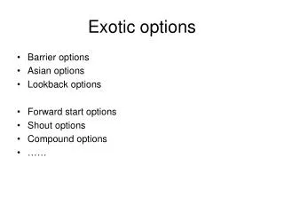
2. Types of Exotics • Package • Nonstandard American options • Forward start options • Compound options • Chooser options • Barrier options • Binary options • Lookback options • Shout options • Asian options • Options to exchange one asset for another • Options involving several assets

3. Packages • Portfolios of standard options • Examples: bull spreads, bear spreads, straddles, etc • Often structured to have zero cost: One popular package is a range forward contract

4. Range Forward Contract Payoff Payoff Asset price K2 K1 K1 K2 Asset price Short Range Forward Contract Long Range Forward Contract

5. Non-Standard American Options • Exercisable only on specific dates (Bermudans) • Early exercise allowed during only part of life (initial “lock out” period) • Strike price changes over the life (warrants, convertibles)

6. Forward Start Options • Option starts at a future time, T1 • Most common in employee stock option plans • Often structured so that strike price equals asset price at time T1

7. Compound Option • Option to buy or sell an option • Call on call • Put on call • Call on put • Put on put • Can be valued analytically • Price is quite low compared with a regular option

8. Chooser Option “As You Like It” • Option starts at time 0, matures at T2 • At T1 (0 < T1 < T2) buyer chooses whether it is a put or call • This is a package!

9. Chooser Option as a Package • At time T1, the value is max(c,p) • From put-call parity, • The value at time T1 is therefore • Package: a call maturing at time T2 plus put with strike maturing at time T1.

10. Barrier Options • Option comes into existence only if stock price hits barrier before option maturity • ‘In’ options • Option dies if stock price hits barrier before option maturity • ‘Out’ options

11. Barrier Options (Cont’d) • Stock price must hit barrier from below • ‘Up’ options • Stock price must hit barrier from above • ‘Down’ options • Option may be a put or a call • Eight possible combinations

12. Parity Relations • c = cui + cuo • c = cdi + cdo • p = pui + puo • p = pdi + pdo

13. Binary Options • Cash-or-nothing: pays Q if ST> K, otherwise pays nothing. • Value = e–rT QN(d2) • Asset-or-nothing: pays ST if ST> K, otherwise pays nothing. • Value = S0N(d1)

14. Decomposition of a Call Option Long Asset-or-Nothing option Short Cash-or-Nothing option where payoff is K Value = S0N(d1) – e–rT KN(d2)

15. Lookback Options • Lookback call pays ST – Smin at time T • Allows buyer to buy stock at lowest observed price in some interval of time • Lookback put pays Smax– STat time T • Allows buyer to sell stock at highest observed price in some interval of time • Analytic solution

16. Shout Options • Buyer can ‘shout’ once during option life • Final payoff is either • Usual option payoff, max(ST – K, 0), or • Intrinsic value at time of shout, St – K • Payoff: max(ST – St , 0) + St – K • Similar to lookback option but cheaper • How can a binomial tree be used to value a shout option?

17. Asian Options • Payoff related to average stock price • Average Price options pay: • Call: max(Save – K, 0) • Put: max(K – Save , 0) • Average Strike options pay: • Call: max(ST – Save , 0) • Put: max(Save – ST , 0)

18. Arithmetic Asian Options • No analytic solution • Can be valued by assuming (as an approximation) that the average stock price is lognormally distributed

19. Exchange Options • Option to exchange one asset for another • For example, an option to exchange one unit of U for one unit of V • Payoff is max(VT – UT, 0) where

20. Basket Options • Monte Carlo Simulation: Perhaps the most commonly used method of pricing basket options. • Although not computationally efficient (particularly as the number of underlying assets is large), Monte Carlo has the ability of handling numerous assets which otherwise would be difficult to evaluate under analytical, tree or finite difference models. • By simulating each underlying asset and then discounting the associated payoff of the basket option, we know that a solution can be reached.

21. Basket Options (Cont’d) • As with all other multi-asset problems pricing basket options requires one to decompose the correlation matrix: 1) Determine a suitable correlation matrix for the underlying assets.2) Set up a simulation for the paths.3) Generate random normal variables with mean of 0 and variance of 1.4) Standardize the variables.5) Apply Cholesky decomposition – but noting that some correlation values cannot be used as they are not positive.6) For each path, loop the simulations from 0 to n and 0 to i, where n is the number of underlying assets and i represent the number of time periods.

22. How Difficult is it to Hedge Exotic Options? • In some cases exotic options are easier to hedge than the corresponding vanilla options. (e.g., Asian options) • In other cases they are more difficult to hedge (e.g., barrier options)

23. Static Options Replication • This involves approximately replicating an exotic option with a portfolio of vanilla options • Underlying principle: if we match the value of an exotic option on some boundary , we have matched it at all interior points of the boundary • Static options replication can be contrasted with dynamic options replication where we have to trade continuously to match the option

24. Example • A 9-month up-and-out call option an a non-dividend paying stock where S0 = 50, K = 50, the barrier is 60, r = 10%, and s = 30% • Any boundary can be chosen but the natural one is c (S, 0.75) = MAX(S – 50, 0) when S< 60 c (60, t ) = 0 when 0 £t£ 0.75

25. Using Static Options Replication • To hedge an exotic option we short the portfolio that replicates the boundary conditions • The portfolio must be unwound when any part of the boundary is reached

26. Boundary Points S C B 60 x x x D A 50 t 0.25 0.50 0.75

27. Example (Cont’d) • We might try to match the following points on the boundary over the life of the option into a number of time steps c(S , 0.75) = MAX(S – 50, 0) for S< 60 c(60, 0.50) = 0 c(60, 0.25) = 0 c(60, 0.00) = 0

28. Black-Scholes European Options • A: 9-month European call option with strike price 50; Position = 1 • B: 9-month European call option with strike price 60; A and B worth when S = 60 at 6-month point 11.54 (A), 4.33 (B); Position = 11.54/-4.33 = -2.66 • C: 6-month European call option with strike price 60; C worth 4.33 when S = 60 at 3-month point; A & B worth -4.18 when S = 60 at 3-month point; Position = -4.18/-4.33 = 0.97 • D: 3-month European call option with strike price 60; To match the secondary boundary condition at time 0; A & B & C = -1.21. D at the 0-time point worth 4.33. Position = -1.21/-4.33 = 0.28

29. Static Hedge – S = 60 at 6-month point

30. Static Hedge – S = 60 at 3-month point

31. Static Hedge – S = 60 at 0-time point

32. European Call Used to Replicate an Up-and-Out Option – S = 50 at 0-time point

33. Example (Cont’d) We can do this as follows: +1.00 call with maturity 0.75 & strike 50 –2.66 call with maturity 0.75 & strike 60 +0.97 call with maturity 0.50 & strike 60 +0.28 call with maturity 0.25 & strike 60

34. Example (Cont’d) • This portfolio is worth 0.73 at time zero compared with 0.31 for the up-and out option • As we use more options the value of the replicating portfolio converges to the value of the exotic option • For example, with 18 points matched on the horizontal boundary the value of the replicating portfolio reduces to 0.38; with 100 points being matched it reduces to 0.32

35. Parisian Options • Parisian options are essentially a crossover between barrier options and Asian options. They have predominant barrier option features in that they can be knocked in or out depending on hitting a barrier from under or above; they differ from standard barrier options in that extreme outlier asset movements will not trigger the Parisian, and for the trigger to be activated or extinguished, the asset must lie outside or inside the barrier for a predetermined time period t. • For example, an up-and-out Parisian call option becomes extinguished if the underlying asset remains above a predetermined barrier level for a prescribed amount of time. Compared to standard barrier options, it can be more beneficial for the holder of a Parisian option on a volatile asset.

36. Uses of Parisian Options • To reduce the incentive for market manipulation that arises with the barrier options. • Apply to model bank deposit guarantees. • Apply to model some U.S. bankruptcy Chapter 11 provisions and to build an ad hoc default framework.

37. Parisian Options -- Introduction • Because of its highly path-dependent nature, Parisian options cannot be solved via a closed form method and common methods involve the consideration of the PDE and the use of a Laplace transform and solving via finite difference methods. The classic paper on pricing Parisian options under continuous monitoring is that of Chesney, Jeanblanc-Picque, Yor (1995) who show the evaluation of the Laplace transform followed by a rapid inversion via the Euler method - also see Hartley (2000).

38. Parisian Options – Introduction (cont’d) • Cornwall & Kentwell (1995) extended Chesney, Jeanblanc-Picque & Yor's (1995) approach to a quasi-analytical model and also incorporating discrete time monitoring, which is actually more often the case in actual markets for Parisian options. • Andersen and Brotherton-Ratcliffe (1996) valued the Parisian options by Monte Carlo Simulations. However, there is a bias linked to the choice of discretisation in the Monte Carlo algorithm.

39. The Partial Differential Equation • Like many other path dependent exotics, solving the PDE on a lattice using finite differences is generally the most reliable method, and in the case of Parisians and barriers, this is even more so the case. • For these options, there are 16 differential equations governing the various cases in which a Parisian can take. Considering all the combinations of down, up, in & out Parisian calls and puts, and then assessing whether the asset price is below or above the strike price, we are able to determine the equations.

40. The Partial Differential Equation (Cont’d) • By considering a three dimensional problem (time, price and duration of out/in), one can solve the PDE via finite differences on a lattice - see e.g. Haber, Schonbucher, Wilmott (1999), Vetzal & Forsyth (1999) and Zhu & Stokes (1999). • Zhu & Stokes use finite element schemes to numerically evaluate the Parisian option and shows that convergence and accuracy of this method can be relied upon when pricing these options.

41. Binomial Trees • By starting off with our basic Cox, Ross, Rubinstein (1979) framework, a binomial tree can incorporate Parisian options by counting the number of nodes in which the Parisian has satisfied its duration condition and determining the price at the node. Note that the term 'duration' merely represents the window it must remain above the barrier for the Parisian to become extinguished. For example, an up-and-out Parisian call option which has a duration of 10 days. Given the up-and-out Parisian having a strike price of 100, a barrier level of 105 and a window period of 10 days, as long as the underlying does not remain above a level of 105 for a period of 10 days, the option remains active

42. Quasi-analytic Solution -- Bernard, Courtois and Quittard-Pinon Procedure • Chesney, Jeanblanc, and Yor (1997) offer an analytic formula based on Laplace transform inversion. However, inverting a Laplace function exactly is in general not possible. Other numerical methods for Parisian options (PDE, Monte Carlo simulations, lattice) are slow to yield precise results. • Bernard, Courtois, and Quittard-Pinon introduced an efficient numerical procedure to approximate the inverse Laplace transform. We therefore discuss their procedure here.

43. The Model • T = maturity of the option • K = strike price • L = barrier level • D = activation or deactivation window • The Parisian option is activated or deactivated if the underlying spends more than D beyond the threshold L. • The underlying stock price is of Black-Scholes diffusion • Define: last time before t that the process S reaches L • Define the first time the underlying S remains more than D below L

44. Sample Excursion Path D S0=95 L=90 T time 0 t

45. Down-and-In Parisian Call Option • By standard arbitrage arguments, the price of a down-and-in Parisian call option • If • If for S0 > L where (S0)=ln(K/S0)/, m=(r-q-2/2)/ and b= ln(L/S0)/.

46. PDF of Brownian Excursion • The PDF for Brownian excursion, say, where and  is law of • Problem: Impossible to obtain a closed-form expression either of h1 or for h2.

47. Laplace Transform • The Laplace transform is an integral transform perhaps second only to the Fourier transform in its utility in solving physical problems. The Laplace transform is particularly useful in solving linear ordinary differential equations such as those arising in the analysis of electronic circuits. • The (unilateral) Laplace transform is defined by • The inverse Laplace transform is known as the Bromwich integral, sometimes known as the Fourier-Mellin integral (see also the related Duhamel’s convolution principle).

48. Analytic Laplace Functions of h1 and h2 • The functions h1 and h2 after Laplace transform admit closed-form expressions and where and N(.) is the Gaussian cumulative distribution function.

49. Down-and-In Parisian Put Option • By standard arbitrage arguments, the price of a down-and-in Parisian call option • If • If for S0 > L where (S0)=ln(K/S0)/ and b= ln(L/S0)/.

50. Down-and Out Parisian Puts • Parity Relationship: Similar to barrier options. That is, down-and-out + down-and-in = Black and Scholes European option. • For example, where P(S0, T) is the Black-Scholes put.