Download
1 / 41
420 likes | 542 Vues
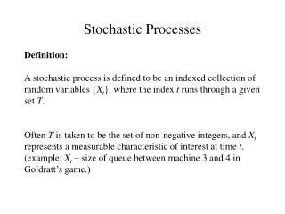
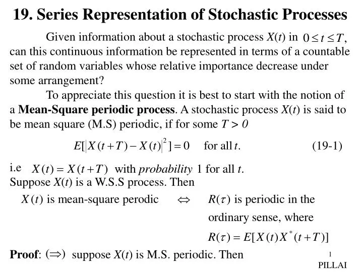
19. Series Representation of Stochastic Processes. Given information about a stochastic process X ( t ) in can this continuous information be represented in terms of a countable set of random variables whose relative importance decrease under some arrangement?

E N D
19. Series Representation of Stochastic Processes Given information about a stochastic process X(t) in can this continuous information be represented in terms of a countable set of random variables whose relative importance decrease under some arrangement? To appreciate this question it is best to start with the notion of a Mean-Square periodic process. A stochastic process X(t) is said to be mean square (M.S) periodic, if for some T > 0 i.e Suppose X(t) is a W.S.S process. Then Proof: suppose X(t) is M.S. periodic. Then (19-1) PILLAI
(19-2) But from Schwarz’ inequality Thus the left side equals or i.e., i.e., X(t) is mean square periodic. (19-3) PILLAI
Thus if X(t) is mean square periodic, then is periodic and let represent its Fourier series expansion. Here In a similar manner define Notice that are random variables, and (19-4) (19-5) (19-6) PILLAI
i.e., form a sequence of uncorrelated random variables, and, further, consider the partial sum We shall show that in the mean square sense as i.e., Proof: But (19-7) (19-8) (19-9) (19-10) PILLAI
and (19-12) Similarly i.e., (19-13) (19-14) PILLAI
Thus mean square periodic processes can be represented in the form of a series as in (19-14). The stochastic information is contained in the random variables Further these random variables are uncorrelated and their variances This follows by noticing that from (19-14) Thus if the power P of the stochastic process is finite, then the positive sequence converges, and hence This implies that the random variables in (19-14) are of relatively less importance as and a finite approximation of the series in (19-14) is indeed meaningful. The following natural question then arises: What about a general stochastic process, that is not mean square periodic? Can it be represented in a similar series fashion as in (19-14), if not in the whole interval say in a finite support Suppose that it is indeed possible to do so for any arbitrary process X(t) in terms of a certain sequence of orthonormal functions. PILLAI
i.e., where and in the mean square sense Further, as before, we would like the cks to be uncorrelated random variables. If that should be the case, then we must have Now (19-15) (19-16) (19-17) (19-18) (19-19) PILLAI
and Substituting (19-19) and (19-20) into (19-18), we get Since (19-21) should be true for every we must have or i.e., the desired uncorrelated condition in (19-18) gets translated into the integral equation in (19-22) and it is known as the Karhunen-Loeve or K-L. integral equation.The functionsare not arbitrary and they must be obtained by solving the integral equation in (19-22). They are known as the eigenvectors of the autocorrelation (19-20) (19-21) (19-22) PILLAI
function of Similarly the set represent the eigenvalues of the autocorrelation function. From (19-18), the eigenvalues represent the variances of the uncorrelated random variables This also follows from Mercer’s theorem which allows the representation where Here and are known as the eigenfunctions and eigenvalues of A direct substitution and simplification of (19-23) into (19-22) shows that Returning back to (19-15), once again the partial sum (19-23) (19-24) (19-25) PILLAI
in the mean square sense. To see this, consider We have Also Similarly (19-26) (19-27) (19-28) (19-29) PILLAI
and Hence (19-26) simplifies into i.e., where the random variables are uncorrelated and faithfully represent the random process X(t) in provided satisfy the K-L. integral equation. Example 19.1: If X(t) is a w.s.s white noise process, determine the sets in (19-22). Solution: Here (19-30) (19-31) (19-32) (19-33) PILLAI
and can be arbitrary so long as they are orthonormal as in (19-17) and Then the power of the process and in that sense white noise processes are unrealizable. However, if the received waveform is given by and n(t) is a w.s.s white noise process, then since any set of orthonormal functions is sufficient for the white noise process representation, they can be chosen solely by considering the other signal s(t). Thus, in (19-35) (19-34) (19-35) (19-36) PILLAI
and if Then it follows that Notice that the eigenvalues of get incremented by q. Example19.2:X(t) is a Wiener process with In that case Eq. (19-22) simplifies to and using (19-39) this simplifies to (19-37) (19-38) (19-39) (19-40) PILLAI
Derivative with respect to t1 gives [see Eqs. (8-5)-(8-6), Lecture 8] or Once again, taking derivative with respect to t1, we obtain or and its solution is given by But from (19-40) (19-41) (19-42) (19-43) PILLAI
and from (19-41) This gives and using (19-44) we obtain Also (19-44) (19-45) (19-46) (19-47) PILLAI
Further, orthonormalization gives Hence with as in (19-47) and as in (19-16), (19-48) (19-49) PILLAI
is the desired series representation. Example 19.3: Given find the orthonormal functions for the series representation of the underlying stochastic process X(t) in 0 < t < T. Solution: We need to solve the equation Notice that (19-51) can be rewritten as, Differentiating (19-52) once with respect to t1, we obtain (19-50) (19-51) (19-52) PILLAI
Differentiating (19-53) again with respect to t1,we get or (19-53) PILLAI
or or Eq.(19-54) represents a second order differential equation. The solution for depends on the value of the constant on the right side. We shall show that solutions exist in this case only if or In that case Let and (19-54) simplifies to (19-54) (19-55) (19-56) (19-57) PILLAI
General solution of (19-57) is given by From (19-52) and Similarly from (19-53) and Using (19-58) in (19-61) gives (19-58) (19-59) (19-60) (19-61) (19-62) PILLAI
or and using (19-58) in (19-62), we have or Thus are obtained as the solution of the transcendental equation (19-63) (19-64) PILLAI
which simplifies to In terms of from (19-56) we get Thus the eigenvalues are obtained as the solution of the transcendental equation (19-65). (see Fig 19.1). For each such the corresponding eigenvector is given by (19-58). Thus since from (19-65) and cn is a suitable normalization constant. (19-65) (19-66) (19-67) (19-68) PILLAI
Karhunen – Loeve Expansion for Rational Spectra [The following exposition is based on Youla’s classic paper “The solution of a Homogeneous Wiener-Hopf Integral Equation occurring in the expansion of Second-order Stationary Random Functions,” IRE Trans. on Information Theory, vol. 9, 1957, pp 187-193. Youla is tough. Here is a friendlier version. Even this may be skipped on a first reading. (Youla can be made only so much friendly.)] Let X(t) represent a w.s.s zero mean real stochastic process with autocorrelation function so that its power spectrum is nonnegative and an even function. If is rational, then the process X(t) is said to be rational as well. rational and even implies (19-69) (19-70) PILLAI
The total power of the process is given by • and for P to be finite, we must have • The degree of the denominator polynomial • must exceed the degree of the numerator polynomial • by at least two, • and • must not have any zeros on the real-frequency • axis. • The s-plane extension of is given by • Thus • and the Laplace inverse transform of is given by (19-71) (19-72) (19-73) PILLAI
Let represent the roots of D(– s2) . Then Let D+(s) and D–(s) represent the left half plane (LHP) and the right half plane (RHP) products of these roots respectively. Thus where This gives Notice that has poles only on the LHP and its inverse (for all t > 0) converges only if the strip of convergence is to the right (19-74) (19-75) (19-76) (19-77) (19-78) PILLAI
of all its poles. Similarly C2(s) /D–(s) has poles only on the RHP and its inverse will converge only if the strip is to the left of all those poles. In that case, the inverse exists for t < 0. In the case of from (19-78) its transform N(s2) /D(–s2) is defined only for (see Fig 19.2). In particular, for from the above discussion it follows that is given by the inverse transform of C1(s) /D+(s). We need the solution to the integral equation that is valid only for 0 < t < T. (Notice that in (19-79) is the reciprocal of the eigenvalues in (19-22)). On the other hand, the right side (19-79) can be defined for every t. Thus, let strip of convergence for Fig 19.2 (19-79) (19-80) PILLAI
and to confirm with the same limits, define This gives and let Clearly and for t > T since RXX(t) is a sum of exponentials Hence it follows that for t > T, the function f (t) must be a sum of exponentials Similarly for t < 0 (19-81) (19-82) (19-83) (19-84) (19-85) PILLAI
and hence f (t) must be a sum of exponentials Thus the overall Laplace transform of f (t) has the form where P(s) and Q(s) are polynomials of degree n – 1 at most. Also from (19-83), the bilateral Laplace transform of f (t) is given by Equating (19-86) and (19-87) and simplifying, Youla obtains the key identity Youla argues as follows: The function is an entire function of s, and hence it is free of poles onthe entire (19-86) (19-87) (19-88) PILLAI
finite s-plane However, the denominator on the right side of (19-88) is a polynomial and its roots contribute to poles of Hence all such poles must be cancelled by the numerator. As a result the numerator of in (19-88) must possess exactly the same set of zeros as its denominator to the respective order at least. Let be the (distinct) zeros of the denominator polynomial Here we assume that is an eigenvalue for which all are distinct. We have These also represent the zeros of the numerator polynomial Hence and which simplifies into From (19-90) and (19-92) we get (19-89) (19-90) (19-91) (19-92) PILLAI
i.e., the polynomial which is at most of degree n – 1 in s2 vanishes at (for n distinct values of s2). Hence or Using the linear relationship among the coefficients of P(s) and Q(s) in (19-90)-(19-91) it follows that are the only solutions that are consistent with each of those equations, and together we obtain (19-93) (19-94) (19-95) (19-96) (19-97) PILLAI
as the only solution satisfying both (19-90) and (19-91). Let In that case (19-90)-(19-91) simplify to (use (19-98)) where For a nontrivial solution to exist for in (19-100), we must have (19-98) (19-99) (19-100) (19-101) PILLAI
The two determinant conditions in (19-102) must be solved together to obtain the eigenvalues that are implicitly contained in the and (Easily said than done!). To further simplify (19-102), one may express akin (19-101) as so that (19-102) (19-103) (19-104) PILLAI
Let and substituting these known coefficients into (19-104) and simplifying we get and in terms of in (19-102) simplifies to if n is even (if n is odd the last column in (19-107) is simply Similarly in (19-102) can be obtained by replacing with in (19-107). (19-105) (19-106) (19-107) PILLAI
To summarize determine the roots with that satisfy in terms of and for every such determine using (19-106). Finally using these and in (19-107) and its companion equation , the eigenvalues are determined. Once are obtained, can be solved using (19-100), and using that can be obtained from (19-88). Thus and Since is an entire function in (19-110), the inverse Laplace transform in (19-109) can be performed through any strip of convergence in the s-plane, and in particular if we use the strip (19-108) (19-109) (19-110) PILLAI
then the two inverses obtained from (19-109) will be causal. As a result will be nonzero only for t > T and using this in (19-109)-(19-110) we conclude that for 0 < t < T has contributions only from the first term in (19-111). Together with (19-81), finally we obtain the desired eigenfunctions to be that are orthogonal by design. Notice that in general (19-112) corresponds to a sum of modulated exponentials. (19-111) (19-112) PILLAI
Next, we shall illustrate this procedure through some examples. First, we shall re-do Example 19.3 using the method described above. Example 19.4: Given we have This gives and P(s), Q(s) are constants here. Moreover since n = 1, (19-102) reduces to and from (19-101), satisfies or is the solution of the s-plane equation But |esT| >1 on the RHP, whereas on the RHP. Similarly |esT| <1 on the LHP, whereas on the LHP. (19-113) (19-114) PILLAI
Thus in (19-114) the solution s must be purely imaginary, and hence in (19-113) is purely imaginary. Thus with in (19-114) we get or which agrees with the transcendental equation (19-65). Further from (19-108), the satisfy or Notice that the in (19-66) is the inverse of (19-116) because as noted earlier in (19-79) is the inverse of that in (19-22). (19-115) (19-116) PILLAI
Finally from (19-112) which agrees with the solution obtained in (19-67). We conclude this section with a less trivial example. Example 19.5 In this case This gives With n = 2, (19-107) and its companion determinant reduce to (19-117) (19-118) (19-119) PILLAI
or From (19-106) Finally can be parametrically expressed in terms of using (19-108) and it simplifies to This gives and (19-120) (19-121) PILLAI
and and substituting these into (19-120)-(19-121) the corresponding transcendental equation for can be obtained. Similarly the eigenfunctions can be obtained from (19-112). PILLAI