Download
1 / 37
380 likes | 618 Vues
The Fresnel Imager for exoplanet study. Laurent Koechlin 1 , Jean-Pierre Rivet 2 , Truswin Raksasataya 1 , Paul Deba 1 , Denis Serre 3. 1 Université de Toulouse CNRS 2 Observatoire de la c ôte d'Azur CNRS 3 Leiden University, the Netherlands. I. Concept.

E N D
The Fresnel Imager for exoplanet study Laurent Koechlin 1, Jean-Pierre Rivet 2, Truswin Raksasataya 1, Paul Deba 1, Denis Serre 3. 1 Université de Toulouse CNRS 2 Observatoire de la côte d'Azur CNRS 3 Leiden University, the Netherlands
Lens (or miror): focusing by refraction (or reflexion) focus Plane wavefront Fresnel array: focusing by diffraction … focus Optical concept: Light focalization Lens Spherical wavefront Binary transmission function g(x) Order 0 : plane wave Order 1 : convergent
Optical concept : Image formation Can light travel free in vacuum all the way from source to focus? Image Aperture Quasi no stray light except in four spikes. Transmission: g(x) Transmission: g(x)"xor" g(y) non linear luminosity scale, to show the spikes.
Basic concepts: Fresnel arrays versus solid aperture Images of a point source by: 300 Fresnel zones 3000 Fresnel zones Solid square aperture luminosity scale:Power 1/4 to show spikes
Basic concepts: Dynamic range & resolution PSF for 300 zones (720 000 apertures) Numerical Fresnel propagation apodized prolate, order 0 masked Log dynamic 1/4 field represented Position in the field (resels)
"Against" Fresnel Arrays: f Chromaticity... But can be canceled by order -1 chromaticityafter focus, Channel bandpass limitations: Δλ/λ= 15% f = D2/8zλ D transmission efficiency to focus: 6% to 10% 1km to 100km focal lengths => Formation flying in space f = D2/8zλ
"pro" Fresnel Arrays: No mirror, no lens : just vacuum and opaque material (except near focal plane). broad spectral domain: λ = 90nm (UV) to (IR) 25μm High angular resolution: as a solid aperture the size of the array. High dynamic range: 108 on compact objects, more with coronagraphy & postprocessing. Large tolerance in positioning of subapertures: for λ/50 wavefront quality in the UV on a 30 meters membrane array: 50 μm in the plane of the membrane, 10 mm perp. to membrane, The tolerance is wavelength independent. Opens the way to large (up to 100m?) aberration-free apertures.
II. Tests Does it work ?
2x2 cm array I have it here, It's working. live demo after this session. For those who Haven't already Seen it…
8x8 cm array: tests on lab sources (2005-2008) 116 zones, 8 x 8 cm 26680 apertures "orthocircular" design. F= 23 m at = 600 nm Precision: 5m on holes positioning =>/70 on wavefront. Achievements: Diffraction limited Broad band imaging (450-850nm) 10-6dynamic range metal foil 100 m thick Photo T.Raksasataya
20x20 cm array: test on sky sources (2009-2011) 0.8" resolution 1000x1000 field λ0 = 800 nm Δλ = 100 nm Photo D.Serre
Metal foil 9.7 105 apertures, Slightly apodized, 696 Fresnel zones. 20 cm Photo P.Deba
20x20 cm array: first light on stars ALINEMENT PHASE images: temporary 116 zones secondary (instead of 702 zones) Tip-Tilt not yet implemented 52 Cygni a-b Va= 4.2 vb= 8.7 sep= 6.4" STT 433 a-b Va=4.36 ; Vb=10.0 Sep= 15" more results at our workshop in Nice next week
20 cm array goals Assess performances on real sky objects: do better than other 20 cm aperture instruments. Targets: High contrast objects extended sources dense fields deep sky
ESA study ESA call for Feasibility study of a membrane telescope 350 k€
III. Space Mission Science ? Credibility ?
The Fresnel Imager Space Mission 3m to 100m diameter, or more. Thin membrane "Primary Array" module: Field optics telescope 1/10th to 1/20th the diameter of Primary Array. Dispersion correction: order -1 diffraction Blazed lens or concave grating, 10 to 30 cm diameter focal Instrumentation: Spectro-imagers
Rationale Meet acceptability threshold for a new technology mission Make it simple, try to keep cost below 300 M€ Scientific return over cost:must be higher than that ofcompeting concepts λ/50 wavefront, at any λ => High Dynamic range from IR to UV mas angular resolution 1000x1000 resel. fields Spectral resolution Suitable for Exoplanets and other fieds too…
Strategy, sky targets - Start with UV domain? - limited budget => limited aperture, but high resolution - High quality wavefront at any wavelength - angular resolution : 7 mas with a 4m Fresnel array - spectral lines in UV for: Photosynthesis break, O3, CH4, CO2 , auroras … - polarimetry
Space Mission: optical scheme Spacecraft 1 Solar Baffle, to protect from sunlight Large "Primary Fresnel Array: Thin foil, 4 to 30 m diameter, or more. Field optics telescope Order zero blocked Focal instrum. Diffraction order 1: focused, but with chromatic aberration. Spacecraft 2 pupil plane Diffraction order 0: unfocussed will be focused by field optics, then blocked. Focal instruments Chromatic correction: Blazed Fresnel grating 5 km (for a 4m aperture) to 100 km (for a 30m aperture) image plane 1dispersed image plane 2 achromatic
Targets: S/N on exoplanets in UV Signal / noise as a function of uv uv Signal / noise > 30 0.5 Jupiter diameter 1 Jupiter diameter planet Signal / noise > 3 Signal / noise < 3 Signal / noise > 3 Signal / noise < 3 Images & spectra of exoplanets: 1 UA from solar type star, 10Pc away 4m aperture, 10h integration spectral res. /= 50 dynamic range of raw image: 2 10^-8
Conclusion Build up a proposal for a 2020 / 2025 launch Science cases: Exoplanets, and also stellar physics compact objects reflection nebulae extragalactic solar system objects observation of the earth 21/2 days workshop in Nice, Sept. 23-25 (next week) Free registration Web site:search with key words "fresnel imager Nice" http://www.ast.obs-mip.fr/users/lkoechli/w3/space_borne_page/page_congres.html We are starting a "Fresnel Imager Astro Applications" group.
Thank you for your attention! You are welcome to join us. Workshop: sept 23-25 (next week)
Optical concept : Image formation Circular Fresnel Zone Plate => PSF with isotropic rings Image Aperture Isotropic rings non linear luminosity scale to show the rings.
expansion 2D Cartésienne Réseau de Fresnel ou Interféromètre à forte densité d’ouvertures ? Géométrie "orthogonale pure" (2005) 4 % de la lumière focalisée 1740 motifs individuels Géométrie "ortho-circulaire" (2008) 6 % de la lumière focalisée
Chromatically aberrated beam at prime focus The field vs spectral bandpas tradeoff Field delimited by field mirror The chromatic corrector does a good job, but it corrects only what it collects.
Fresnel Imager specifications UV spectro-Imaging at High Dynamic Range 4m aperture 3 spectral bands Δλ/λ=20%: 2 in the UV, 1 in the visible λ/50 wavefront spectral resolution λ/δλ=50 angular resolution 7 to 25 mas depending on λ field 1000x1000 => 7 to 25 arc seconds raw dynamic range >108 - with 10 hours integrations time: jovian exoplanets with apertures of 1 m or more telluric Exoplanets: only with 10 meters apertures or larger - Other fields of astrophysics
Gen III prototype: Primary array R&T financed by CNES & STAE Size : 8 cm, square 240 Fresnel zones (110 000 apertures) metal sheet 100 m thick, laser carved Operates in the UV (250-350 nm) Focal length: 26.6 m for = 250 nm Precision on array : 5m i.e./30 on wavefront
Gen III prototype Critical point: concave blazed mirror infocal module
Orbites et pointages petite Lissajou periode : 6 mois1 eclipse en 6 ans, évitable Lingne de visée eclipticque Fresnel baffle sun sun 200 000 km Terre éclipticque L2 8° 14° Lune • Seul, Lagrange L2 répond à tous les besoins: • pas de gradient de gravité sur une grande base • masquage du soleil et de la Terre dans un angle réduit • bonne liberté de pointage • Pour la très haute dynamique: nécessité de masquer toute lumière parasite avec taille pare soleil réduit et possibilité de dépointage acceptable: • 35% de la voûte à tout instant, 100% en 4 mois. • implique petite ou moyenne orbite de Lissajou Antenne RA fixe et GS fixe possible à partir de 100 000km de la Terre
Résultats qualitatifs : dynamiquemesure optiqueet simulation numérique Dans ces images d'un point, saturées, le fond moyen est à 2 *10 -6 Luminosité amplifiée x1000 Luminosité amplifiée x1000 8 cm 116 zones image Optique 8 cm 116 zones propagation de Fresnel numerique par tous les éléments optiques propagation numerique de Fresnel développée pour tester de grands réseaux
expansion 2D Cartésienne Réseau de Fresnel ou Interféromètre à forte densité d’ouvertures ? Géométrie "orthogonale pure" (2005) 4 % de la lumière focalisée 1740 motifs individuels Géométrie "ortho-circulaire" (2008) 6 % de la lumière focalisée