Download
1 / 39
390 likes | 502 Vues
Speciation Dynamics of an Agent-based Evolution Model in Phenotype Space. Adam D. Scott Center for Neurodynamics Department of Physics & Astronomy University of Missouri – St. Louis. Oral Comprehensive Exam 5*31*12. Proposed Chapters.

E N D
Speciation Dynamics of an Agent-based Evolution Model in Phenotype Space Adam D. Scott Center for Neurodynamics Department of Physics & Astronomy University of Missouri – St. Louis Oral Comprehensive Exam 5*31*12
Proposed Chapters • Chapter 1: Clustering and phase transitions on a neutral landscape (completed) • Chapter 2: Simple mean-field approximation to predict universality class & criticality for different competition radii • Chapter 3: Scaling behavior with lineage and clustering dynamics
Basis Biological • Modeling • Phenotype space with sympatric speciation • Phenotype = traits arising from genetics • Sympatric = “same land” / geography not a factor • Possibility vs. prevalence • Role of mutation parameters as drivers of speciation • Evolution = f(evolvability) • Applicability Physics & Mathematics • Branching & Coalescing Random Walk • Super-Brownian • Reaction-diffusion process • Mean-field & Universality • Directed &/or Isotropic Percolation
Broader Context/ Applications • Bacteria • Example: microbes in hot springs in Kamchatka, Russia • Yeast and other fungi • Reproduce sexually and/or asexually • Nearest neighbors in phenotype space can lead naturally to assortative mating • Partner selection and/or compatibility most likely • MANY experiments involve yeast
Model: Overview • Agent-based, branching & coalescing random walkers • “Brownian bugs” (Young et al 2009) • Continuous, two-dimensional, non-periodic phenotype space • traits, such as eye color vs. height • Reproduction: Asexual fission (bacterial), assortative mating, or random mating • Discrete fitness landscape • Fitness = # of offspring • Natural selection or neutraldrift • Death: coalescence, random, & boundary
Model: “Space” • Phenotype space (morphospace) • Planar: two independent, arbitrary, and continuous phenotypes • Non-periodic boundary conditions • Associated fitness landscape
Model: Fitness Natural Selection Neutral Theory Hubbell Ecological drift Kimura Genetic drift Equal (neutral) fitness for all phenotypes No deterministic selection Random drift Random selection Fitness = 2 • Darwin • Varying fitness landscape over phenotype space • Selection of most fit organsims • Applicable to all life • Fitness = 1-4 • (Dees & Bahar 2010)
Model: Mutation Parameter • Mutation parameter -> mutability • Ability to mutate about parent(s) • Maximum mutation • All organisms have the same mutability • Offspring uniformly generated Example of assortative mating assuming monogamous parents
Model: Reproduction Schemes • Assortative Mating • Nearest neighbor is mate • Asexual Fission • Offspring generation area is 2µ*2µ with parent at center • Random Mating • Randomly assigned mates
Model: Death • Coalescence • Competition • Offspring generated too close to each other (coalescence radius) • Random • Random proportion of population (up to 70%) • “Lottery” • Boundary • Offspring “cliff-jumping”
Model: Clusters • Clusters seeded by nearest neighbor & second nearest neighbor of a reference organism • A closed set of cluster seed relationships make a cluster = species • Speciation • Sympatric Cluster seed example: The white organism has nearest neighbor, yellow (solid white line). White’s 2nd nearest neighbor is blue (hashed white line). Therefore, white’s cluster seed includes: white, yellow, and blue.
Generations 00.40 1 50 1000 2000 00.44 µ 00.50 01.20
Chapter 1: Neutral Clustering & Phase Transitions • Non-equilibrium phase transition behavior observed for assortative mating and asexual fission, not for random mating • Surviving state clustering observed to change behavior above criticality
Assortative Mating • Potential phase transition • Extinction to Survival • Non-equilibrium • Extinction = absorbing • Critical range of mutability • Large fluctuations • Power-law species abundances • Peak in clusters Quality (Values averaged over surviving generations, then averaged over 5 runs)
Asexual Fission • Slightly smaller critical mutability • Same phase transition indicators • Same peak in clusters • Similar results for rugged landscape with Assortative Mating
Control case: Random mating Generations 1 50 1000 2000 02.00 µ 07.00 12.00
Random Mating • Population peak driven by mutability & landscape size comparison • No speciation • Almost always one giant component • Local birth not guaranteed!
Conclusions • Mutability -> control parameter • Population as order parameter • Continuous phase transition • extinction = absorbing state • Directed percolation universality class? • Speciation requirements • Local birth/ global death (Young, et al.) • Only phenotype space (compare de Aguiar, et al.) • For both assortative mating and asexual fission
Chapter 1: Progress • Manuscript submitted to the Journal of Theoretical Biology on April 16 • Under review as of May 2 • No update since
Chapter 2 • Goal: to have a tool which predicts critical mutability and critical exponents for a given coalescence radius = Mean-field equation • Directed percolation (DP) & Isotropic percolation (IP) • Neutral landscape with fitness = 2 for all phenotypes • May extend to arbitrary fitness if possible • Asexual reproduction • Will attempt extension to assortative mating
Temporal & Spatial Percolation • Temporal Survival • Time to extinction becomes computationally infinite • DP • Spatial “Space filling” • Largest clusters span phenospace • IP
1+1 Directed Percolation • Reaction-diffusion process of particles • Production: A2A • Coalescence: 2AA • Death: A0 • Offspring only coalesce from neighboring parent particles N N+1 Death (A→ᴓ) Production(A→2A) Coalescence (2A →A)
Chapter 2: Self-coalescence • Not explicitly considered in basic 1+1 DP lattice model • Mimics diffusion process • May act as a correction to fitness, giving effective birth rate • “Sibling rivalry” • Probability for where the first offspring lands in the spawn region • Probability that the second offspring lands within a circle of a given radius whose center is offspring one and its area is also in the spawn region 2 1
Chapter 2: Neighbor Coalescence • Offspring from neighboring parents coalesce Coalescence (2A →A) 2 1 1 2
Assuming Directed Percolation • Simple mean-field equation (essentially logistic) • Density as order parameter • τ is the new control parameter • should depend on mutability and coalescence radius • is effective production rate (fitness & self-coalescence) • is effective death rate (random death) • g is a coupling term • g = , the effective coalescence rate (”neighbor rivalry”)
Chapter 2: Neutral Bacterial Mean-field • Birth: • Coalescence: • Random death: • Effective production rate = • Effective death rate = • Effective coalescence rate = ? • Possibly a coupled dynamical equation for nearest neighbor spacing • & • Without nc, current prediction for critical mutability (~0.30) is <10% from simulation (~0.33)
Chapter 2: Neighbor Coalescence • Increased rate with larger mutability & coalescence radius • Varies amount of overlapping space for coalescence • Should depend explicitly on nearest neighbor distances • May be determined using a nearest neighbor index or density correlation function • Possibility of a second dynamical equation of nearest neighbor measure coupled with density?
Chapter 2: Progress • Have analytical solution for sibling rivalry • Have method in place to estimate neighbor rivalry • Waiting for new data for estimation • Need to finish simple mean-field equation • Need data to compare mean-field prediction of criticality for different coalescent radii • Determine critical exponents • Density, correlation length, correlation time
Chapter 3: Scaling • Can organism behavior predict lineage behavior? • Center of “mass” center of lineage (CL) • Random walk • Path length of descendent organisms & CL • Branching & (coalescing) behavior • Can organism behavior predict cluster behavior? • Center of species (centroids) • Clustering clusters • Branching & coalescing behavior • May determine scaling functions & exponents • Population # of Clusters? • Fractal-like organization at criticality? • Lineage branching becomes fractal? • Renormalization: organisms clusters
Chapter 3: Cluster level reaction-diffusion • Clusters can produce n>1 offspring clusters • AnA (production) • Clusters go extinct • A0 (death) • m>1 or more clusters mix • mAA (coalescence)
Chapter 3: Predictions • Difference of clustering mechanism by reproduction • Assortative mating: organisms attracted (sink driven) • Greater lineage convergence (coalescence) • Bacterial: clusters from blooming (source driven) • Greater lineage branching (production) • Greater mutability produces greater mixing of clusters & lineages • Potential problem: far fewer clusters for renormalization
Chapter 3: Progress • Measures developed for cluster & lineage behavior • Extracted lineage and cluster measures from previous data • Need to develop concrete method for comparing the BCRW behavior between reproduction types • ?
Related Sources • Dees, N.D., Bahar, S. Noise-optimized speciation in an evolutionary model. PLoS ONE5(8): e11952, 2010. • de Aguiar, M.A.M., Baranger, M., Baptestini, E.M., Kaufman, L., Bar-Yam, Y. Global patterns of speciation and diversity. Nature460: 384-387, 2009. • Young, W.R., Roberts, A.J., Stuhne, G. Reproductive pair correlations and the clustering of organisms. Nature412: 328-331, 2001. • HinsbyCadillo-Quiroz, Xavier Didelot, Nicole Held, Aaron Darling, Alfa Herrera, Michael Reno, David Krause and Rachel J. Whitaker. Sympatric Speciation with Gene Flow in Sulfolobusislandicus.PLoS Biology, 2012. • Perkins, E. Super-Brownian Motion and Critical Spatial Stochastic Systems. http://www.math.ubc.ca/~perkins/superbrownianmotionandcriticalspatialsystems.pdf. • Solé, Ricard V. Phase Transitions. Princeton University Press, 2011. • Yeomans, J. M. Statistical Mechanics of Phase Transitions. Oxford Science Publications, 1992. • Henkel, M., Hinrichsen, H., Lübeck, S. Non-Equilibrium Phase Transitions: Absorbing Phase Transitions. Springer, 2009.
µ = 0.38 µ = 0.40 slope ~ -3.4 • Power law distribution of cluster sizes • Scale-free • Large fluctuations near critical point (Solé 2011) • Characteristic of continuous phase transition • Near criticality parabolic distributions change gradually • Mu < critical concave down • Mu > critical concave up µ = 0.42
Clark & Evans Nearest Neighbor Test Asexual Fission Clustered <= 0.46 (peak) Dispersed >= 0.54 Better than 1% significance Assortative Mating • Clustered <= 0.38 (peak) • Dispersed >= 0.44 • Better than 1% significance