Download
1 / 1
10 likes | 80 Vues
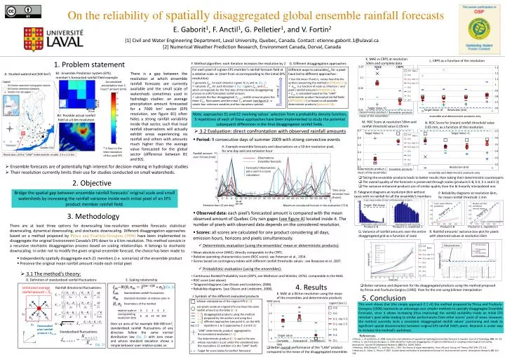
R 1. R 2. R 3. R 4. 2. 3. 1. On the reliability of spatially disaggregated global ensemble rainfall forecasts. E. Gaborit 1 , F. Anctil 1 , G. Pelletier 1 , and V. Fortin 2.

E N D
R1 R2 R3 R4 2 3 1 On the reliability of spatially disaggregated global ensemble rainfall forecasts E. Gaborit1, F. Anctil1, G. Pelletier1, and V. Fortin2 [1] Civil and Water Engineering Department, Laval University, Quebec, Canada. Contact: etienne.gaborit.1@ulaval.ca [2] Numerical Weather Prediction Research, Environment Canada, Dorval, Canada K. MAE vs CRPS at resolution 50km and complete data L. CRPS as a function of the resolution 1. Problem statement F. Method algorithm: each iteration increases the resolution by 2 G. Different disaggregation approaches MAE CRPS For each pixel of a given EPS member’s rainfall forecast field at a relative scale m (start from m corresponding to the initial EPS resolution): Different ways to calculateξm for a pixel have led to different approaches : See J. B1- Ensemble Prediction System (EPS) member’s forecasted rainfall field example There is a gap between the resolution at which ensemble rainfall forecasts are currently available and the small scale of watersheds sometimes used in hydrologic studies: an average precipitation amount forecasted for a 7000 km2 sector (EPS resolution, see figure B1) often hides a strong rainfall variability inside that sector, such that local rainfall observations will actually exhibit areas experiencing no rainfall and others with amounts much higher than the average value forecasted for the global sector (difference between B1 and B2). A- Studied watershed (500 km2) • Use the mean H andσ1 values found by the authors presenting the method (APPROACH E1). • σm,i is a function of scale m, direction i and pixel’s rainfall amount (APPROACH E2). • ξm,iis calculated based on the “LAM” deterministic product forecasted rainfall fields (APPROACH E3) or based on all available deterministic products (approach E4). Accumulated precipitation over 3 hours* amount (mm) • generate ξm,i for each direction igiven H, σ1and m(Eq. 2) • calculate X’m,i for each direction i(Eq. 1) given ξm,i and Xm, which corresponds for the first step of this iterative disaggregating process to a EPS forecasted rainfall amount. • calculate the four disaggregated Rk=1:4rainfall amounts given the three X’m,i fluctuations and the initial Xmamount (see figure D: a simple four unknown variables and four equations system). m=m-1 100 km Target Value =0 Target Value =0 70 km Deterministic product / mean of the ensembles Ensemble products Note: approaches E1 and E2 involving values’ selection from a probability density function, 5 repetitions of each of these approaches have been implemented to study the potential subsequent differences in the final disaggregated rainfall fields. B2- Possible actual rainfall field at a 6 km resolution ensemble and deterministic products only M. ROC Score at resolution 50km and rainfall threshold value 0.05mm N. ROC Score for (mean) rainfall threshold value 0.05 mm, as a function of the resolution • 3.2 Evaluation: direct confrontation with observed rainfall amounts Target Value =1 Target Value =1 See J. • Period: 9 consecutive days of summer 2009 with strong convective events H. Example ensemble forecasts and observations on a 50-km resolution pixel, for one day and one emission hour * 3 hours is the time resolution of the used EPS Rainfall amount over 3 hours (mm) Resolution of the “LAM” deterministic model: 2.5 x 2.5 km Observations Ensemble forecasts • Ensemble forecasts are of potentially high interest for decision-making in hydrologic studies • Their resolution currently limits their use for studies conducted on small watersheds. Forecasts/ Observations pairs used in a score calculation Deterministic product / mean of the ensembles Ensemble products ensemble and deterministic products only • Taking the ensemble products leads to better results than taking their deterministic counterparts • The overall quality of the forecasts is preserved through scales (products E-B, E-0, E-1 and E-2) • The variance-enhanced products are of similar quality than the bi-linearily interpolated one 2. Objective Time since emission hour (hours) O. Talagrand diagrams at resolution 6km without cases with no rainfall for all the ensemble’s members Bridge the spatial gap between ensemble rainfall forecasts’ original scale and small watersheds by increasing the rainfall variance inside each initial pixel of an EPS product member rainfall field. P. Reliability diagrams at resolution 6km, for mean rainfall threshold 1 mm Y axis: mean number of cases with observation in rank n 5 Δt=3h Y axis: mean effective probability Median and 95% confidence interval shown Target: flat shape Emission hour (2 per day) Maximum considered horizon in the evaluation (72 h) 1 Target line • Observed data: each pixel’s forecasted amount is compared with the mean observed amount of Quebec City rain gages (see figure A) located inside it. The number of pixels with observed data depends on the considered resolution. Target line 3. Methodology X axis: nominal probability Observation’s rank n (n=1:22) There are at least three options for downscaling low-resolution ensemble forecasts: statistical downscaling, dynamical downscaling, and stochastic downscaling. Different disaggregation approaches based on a method proposed by Périca and Foufoula-Georgiou (1996) have been implemented to disaggregate the original Environment Canada’s EPS down to a 6 km resolution. This method consists in a recursive stochastic disaggregation process based on scaling relationships. It belongs to stochastic downscaling. In order not to modify the given original ensemble forecast, the choice has been made to: Observation’s rank n (n=1:22) Product E-B Product E-1, repetition 1 Product E-B Product E-1, repetition 1 • Scores: all scores are calculated for one product considering all days, emission hours, horizons and pixels simultaneously. Q. Variance of rainfall amounts over the entire disaggregated grid as a function of scale R. Rainfall amounts’ variance box-plot for pixels with observed values at resolution 6km • Deterministic evaluation (using the ensembles’ mean or deterministic products): Observations 95% boundary See J. 75% boundary median • Mean absolute error (MAE): directly comparable to the CRPS. • Relative operating characteristics score (ROC score): see Peterson et al., 1954. • Scores based on contingency tables with different rainfall thresholds values : see Rezacova et al. 2007. 25% boundary 5% boundary • Independently spatially disaggregate each 21 members (i.e. scenarios) of the ensemble product • Preserve the original mean rainfall amount inside each initial pixel • Probabilistic evaluation (using the ensembles): • 3.1 The method’s theory: • Continuous Ranked Probability score (CRPS, see Matheson and Winkler, 1976): comparable to the MAE. • ROC score (see above). • Talagrand diagrams (see Olsson and Lindström, 2008). • Reliability diagrams (see Olsson and Lindström, 2008). D. Definition of standardized rainfall fluctuations E. Scaling relationship Product 4. Results • Better variance and dispersion for the disaggregated products using the method proposed by Périca and Foufoula-Gergiou (1996) than for the one using bilinear interpolation (Eq. 2) initial pixel average rainfall amount = Xm Rainfall directional fluctuations: Standardized rainfall fluctuations K. MAE at a 06-km resolution using the mean of the ensembles and deterministic products 5. Conclusion J. Symbols of the different evaluated products Standard deviation at relative scale m bilinear interpolation of the original EPS (E-B) MAE (mm) Legend (see J.) Parameters of the method This work shows that (the simple approach E-1 of) the method proposed by Périca and Foufoula-Georgiou (1996) represents an advantage over simpler methods to spatially disaggregate Ensemble Forecasts, since it allows increasing (thus improving) the rainfall variability inside an initial EPS member’s pixel while leading to similar performances from other scores’ point of views. However, the method currently lacks a consistent disaggregated rainfall values’ positioning and leads to significant spatial discontinuities between original EPS rainfall field’s pixels. Research is under way to increase this method’s usefulness. sub-pixels inside an original EPS one have the same rainfall amount as the latter (E-0) E-1 E-2 E-3 E-4 disaggregated products using the method proposed by the authors and using four different approaches (see point G. on the left). Over an area of for example 300 000 km2, standardized rainfall fluctuations of any direction follow the same normal distribution law (Eq. 2) with zero mean and whose standard deviation shows a simple behavior over relative scales m. rep 1:5 repetitions 1 to 5 (approaches E-1 and E-2) Downscaled pixel rainfall amount = Rk=1:4 “LAM” deterministic product aggregated to the considered resolution (D-L) Standardized fluctuations: Target value References The deterministic product (D-T) used is the one whose resolution is just under the considered one (for resolutions 12 and 6km it is the “LAM” itself) • Olsson, J., et Lindström, G. 2008. Evaluation and calibration of operational hydrological ensemble forecasts in Sweden. Journal of Hydrology, 350: 14– 24. • Perica, S., and Foufoula-Georgiou, E. 1996. Model for multiscale disaggregation of spatial rainfall based on coupling meteorological and scaling descriptions. Journal Of GeophysicalResearch, 101(D21): 26347-26361. • Peterson, W.W, Birdsall, T.G., and Fox, W.C., 1954. The theory of signal detectability. Trans. IRE prof. Group. Inf. Theory, PGIT, 2-4: 171-212. • Rezacova, D., Sokol, Z., Pesice, P. 2007. A radar-based verification of precipitation forecast for local convective storms. Atmospheric Research, 83: 211–224. Complete data Forecasts>0 Forecasts=0 (Eq. 1) • Better overall performance of the “LAM” product compared to the mean of the disaggregated ensembles Target for score (value for perfect forecasts)