Download
1 / 26
271 likes | 375 Vues
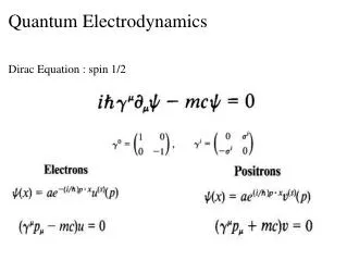
Introduction to Quantum Electrodynamics. Properties of Dirac Spinors Description of photons Feynman rules for QED Simple examples Spins and traces. Summary – Spin-1/2. u (1) , u (2) , v (1) , v (2) need not be pure spin states, but their sum is still “complete”.

E N D
Introduction to Quantum Electrodynamics Properties of Dirac Spinors Description of photons Feynman rules for QED Simple examples Spins and traces Much of the content of these slides is acknowledged to come from “Introduction to Elementary Particles” By David Griffiths, Wiley, 1987
Summary – Spin-1/2 u(1), u(2), v(1), v(2) need not be pure spin states, but their sum is still “complete”. Brian Meadows, U. Cincinnati
Summary - Photons • Photons have two spin projections (s): Brian Meadows, U. Cincinnati
Feynman Rules for QED Label: • Label each external line with 4-momenta p1, … pn. Label theirspins s1, … sn. Label internal lines with 4-momenta q1, … qn Directions: Arrows on external indicate Fermion or anti-Fermion Arrows on internal lines preserve flow Arrows on internal lines preserve flow External photon arrows point in direction of motion Internal photon arrows do not matter Brian Meadows, U. Cincinnati
Feynman Rules for QED • For external lines, write factor • For each vertex write a factor Always follow a Fermion line To obtain a product: (adjoint-spinor)()(spinor) E.g.: pj , sj pk , sk e - e - q u (sk)(k) ige u(s))(j) Brian Meadows, U. Cincinnati
Feynman Rules for QED • Write a propagator factor for each internal line NOTE: qj2 = mj2c2 for internal lines. NOTE also: use of the ”slash – q” a 4 x 4 matrix rather than a 4-vector! Brian Meadows, U. Cincinnati
Feynman Rules for QED Now conserve momentum (at each vertex) 5. Include a d function to conserve momentum at each vertex. where the k's are the 4-momenta entering the vertex 6. Integrate over all internal 4-momenta qj. I.e. write a factor For each internal line. • Cancel the d function. Result will include factor • Erase the d function and you are left with • Anti-symmetrize (“-” sign between diagrams with swapped Fermions) Brian Meadows, U. Cincinnati
p1 , s1 p3 , s3 e - e - u (s3 )(3) ige u(s1 )(1) q u (s4 )(4) ige u(s2 )(2) - - p2 , s2 p4 , s4 NOTE u(k) is short for u(sk )(pk) Example – e-- e--Scattering • We already wrote down one vertex: Use index “” • The other is similar: BUT use index “” • Leads to Brian Meadows, U. Cincinnati
Evaluate – e-- e--Scattering(Griffiths, problem 7:24) • Assume e - and - move along the z-axis, each with helicity +1. After collision, they return likewise. Therefore where Brian Meadows, U. Cincinnati
The electron and muon vertex functions: • So the inner product is Brian Meadows, U. Cincinnati
p1 , s1 p1 , s1 p4 , s4 p3 , s3 e - e - e - e - q q e- p3 , s3 e- e- p2 , s2 e- p2 , s2 p4 , s4 Example – e-e- e-e- (Moller Scattering) • One other diagram required in which 3 4 are interchanged (not possible in e-- scattering) • Anti-symmetrization leads to: Brian Meadows, U. Cincinnati
Spin Summation and Averaging • We have, so far: • Consider e- scattering. To obtain a cross-section or decay rate, we need to evaluate and (usually) sum over final spins and average over initial ones. • Each term in […] is a number, as seen above, so we can re-order them and evaluate in pairs like whereis a 4 x 4 matrix (in this case,). Brian Meadows, U. Cincinnati
Spin Summation and Averaging • It is easy to show that • Therefore we can re-write V with the u(1)’s together: 4 x 4 matrix Brian Meadows, U. Cincinnati
Spin Summation and Averaging • To sum over spins for particle 1, use the completeness property: • Now sum over spins for particle 3: 4 x 4 matrix WHY ? scalar Scalar NO u’s !! Brian Meadows, U. Cincinnati
Spin Summation and Averaging • Why is: • Pre-multiply by u(3) then post-multiply by u(3) • So 4 x 4 matrix scalar ? 4 x 4 matrix Brian Meadows, U. Cincinnati
Spin Summation and Averaging • Repeat for other vertex to get: • For the specific case of e- scattering: where m is mass of electron and M is mass of . Average over 4 initial spins Brian Meadows, U. Cincinnati
Dirac g Matrices - Reminder • Almost done, but we need to use gm,g5, p, etc.. Brian Meadows, U. Cincinnati
… About the Traces • Almost done, but the traces need some ready results: Brian Meadows, U. Cincinnati
Evaluate Traces for e- Scattering • We obtained: • Expand the first factor: Spin average over initial states 4 g 0 0 Brian Meadows, U. Cincinnati
Evaluate Traces for e- Scattering • Therefore • So the first factor is: • The second factor is therefore: Brian Meadows, U. Cincinnati
Evaluate Traces for e- Scattering • The product is: • Contracting terms: • Done with traces! Brian Meadows, U. Cincinnati
e - e - - Evaluate Cross-Section for e- Scattering • Work in the frame where the is at rest. Assume so that we can ignore the recoil of the, and therefore |p1| = |p3| = |p| and |p2| = |p4| = 0 • Computing terms in matrix element: Brian Meadows, U. Cincinnati
Evaluate Cross-Section for e- Scattering • Insert in matrix element: • To get the cross-section: Brian Meadows, U. Cincinnati
Limiting Cases: • Relativistically, we have Mott scattering (originally for e- p): • Low energy we get Rutherford scattering: • High energy limit Brian Meadows, U. Cincinnati
Compton Scattering • Two diagrams in lowest order: • Apply Feynman rules (first diagram – second is similar): p2 , s2 p4 , s4 p2 , s2 p4 , s4 + Time p1 , s1 p3 , s3 p1 , s1 p3 , s3 Fermion line (backwards) g in g out Brian Meadows, U. Cincinnati
Compton Scattering • Conserve energy-momentum, etc.: where q = p1-p3, etc.. • Add term for other diagram. • Write as trace • Evaluate trace • Evaluate cross-section Brian Meadows, U. Cincinnati