Download
1 / 39
390 likes | 552 Vues
Mobile Networking - Part I (Physical Layer). EE206A (Spring 2004): Lecture #2. This + Next Few Lectures. What are the problems in communications caused by mobility of network elements? How do various system layers cope with these problems in traditional mobile networks? We will look at:

E N D
Mobile Networking - Part I(Physical Layer) EE206A (Spring 2004): Lecture #2
This + Next Few Lectures • What are the problems in communications caused by mobility of network elements? • How do various system layers cope with these problems in traditional mobile networks? • We will look at: • Physical layer THIS LECTURE • Link/Network layers • Transport layer • OS/Application layer
Reading List for This Lecture • [REQUIRED] The Mistaken Axioms of Wireless-Network Research. David Kotz, Calvin Newport, Bob Gray, Jason Liu, Yougu Yuan, and Chip Elliot. Technical Report TR2003-467, Dept. of Computer Science, Dartmouth College, July, 2003. http://nesl.ee.ucla.edu/courses/ee206a/sharedp/papers/Kotz04_axioms_mh.pdf (preferred version to read - password protected [see class mailing list]) http://www.cs.dartmouth.edu/~dfk/papers/kotz:axioms-tr.pdf
Shades of Mobility of Network Elements • Terminal moves • Discrete: unplug from one network port, moves elsewhere while disconnected, re-plug at a new network port • Continuous: move terminal with applications unaffected as topology changes • User moves • User moves from terminal to terminal • Infrastructure elements move • Moving basestations - e.g. Iridium satellites, UAVs • Chunks of network moves • Airplane with 802.11 network • Platoon of soldiers
Some Mobility Issues • Terminal speed impacts wireless channel quality • Fading • Terminal and user location • Become system variables of interest • Change dynamically • Constants become variable • Location, environment, connectivity,topology, b/w, I/O devices, security domain • Spoofing becomes easier • Need more of: protocol processing, signal processing, and signaling traffic
Example: Disconnections • Planned vs. unplanned • Choices? • engineer to prevent disconnections • gracefully cope (adapt) to disconnections • Mask disconnections and round-trip latencies • decouple communication from data production/consumption • asynchronous operation (multiple REQs before ACKs), prefetching, delayed write-back etc. • Tolerate by autonomous operation, caching/hoarding, local applications etc. • disconnected filesystems, e.g. CMU’s CODA • Good user interfaces to give feedback about disconnection
Example: Address Migration due to Mobility • Dynamically changing network access point • Network addresses usually correspond to the point of attachment to n/w • applications/calls connect to a fixed address • active connections cannot be moved to new address • How to support changing network access point? • How to find the current address? • How to do rerouting? • How to do route optimization? • How to do multicast?
Example: Location-dependent Information • Location affects configuration parameters • DNS, timezone, printer etc. • Location affects answer to user queries • e.g. where is the nearest printer • More complex location-dependent queries • e.g. where is the nearest taxi • Privacy concerns due to location tracking • Changing context • small movements may cause large changes • caching may become ineffective • dynamic transfer to nearest server for a service • Localization
Mobility and the Physical Layer • Key factor is the wireless link which is impacted by terminal mobility • For network designers, wireless is quite “confusing”! • Does not quite “fit” the wireline paradigm • Breaks down traditional concepts of topology and link quality From Keynote Talk by A. Ephemeredes @ MobiCom 2002
Consequences of being Wireless • Clearly no fixed topology (even without mobility) • Cross-layer coupling • power energy consumption higher/lower layers • other users MAC • rate throughput higher/lower layers • BER other QoS measure application layer • Different world • Rich theory of communications, Complex details • Ignoring the physical layer limits the meaningfulness of upper layers • E.g. disk models of radio range • The notion of “wireless links” is very slippery… From Keynote Talk by A. Ephemeredes @ MobiCom 2002
E.g. of Fluid Notion of Wireless Links: Connectivity & Rate • Lowering the rate permits the packaging of more energy per symbol (SINR > ) • So a faltering link can become more reliable (elasticity) • A previously non-existent link can be created • Rate reduction lowers throughput or increases delay or distorts the signal • Preferable to power because it does not affect interference (non-invasive)
Wireless Link Behavior • Large-scale variations due to T-R distance, obstructions • Small-scale variations due to fading • Three effects: mean path loss, slow variation about the mean, rapid variation • All affected by location and speed!
Path Loss • Path loss is inversely proportional to dn
Path Loss vs. Distance in Free Space • Clear, unobstructed, line of sight • Received power at distance d from sender • where Gt and Gr are antenna gains, L ≥ 1 is a system loss factor due to filter losses, hardware • Path loss = signal attenuation in dB • Model valid only for large d in the “far field” (Fraunhofer Region) of the antenna • D is the largest physical linear dimension of the antenna
Free Space Path Loss in Practice • Use a receive power reference point = d0 • Path loss too expressed in a relative manner
Space with Objects • Reflection (with transmittance and absorbtion) • Objects >> wavelength (e.g. earth, building, atmosperic layers) • Diffraction • Waves bend around sharp edges of impenetrable objects (Huygen’s principle) • A.k.a “shadowing” • Scattering • Objects < wavelength (e.g. foliage , street signs, lamp posts etc.) • Received signal sum of contributions of signals along many different paths
Example: Ground Reflection • For large d >> sqrt (hthr), • Much more rapid path loss with increasing T-R separation
Log-distance Path Loss Model • Path loss exponent n depends on propagation environment and obtained by measurements • Problem: “environment clutter” may differ at two locations at the same d • Measured PL(d) may differ from mean PL(d) • In indoor environments, a floor attenuation factor also added
Log-normal Shadowing Model • Assumes path loss at a given d has a normal distribution • X is a zero-mean gaussian r.v. • says how good the model is • n ~ 2-4, ~ 2-5 dB • Obtained by measurements
More Sophisticated Empirical Models • Log-distance and Log-normal models lump everything into d and • Sophisticated models take into account other factors such as terrain, antenna height, urban clutter etc. • Many outdoor models from cellular industry: Longley-Rice, Durkin, Okumura, Hata etc. • Example: Okumura model for 150-1920 MHz, 1-100 km distances, and 30-1000 m antenna heights
Non-empirical Models • Empirical models provide exact match for system under consideration, but are: • Expensive (due to measurement process) • Hard to generalize (change in frequency, environment) • Non-empirical approaches • Analytic models • e.g. [Xia97] • Ray-tracing models
Link Budget using Path Loss Models • Bit-error-rate is a function of SNR (signal-to-noise ratio), or equivalently CIR (carrier-to-interference ratio), at the receiver • the “function” itself depends on the modulation scheme! • Link budget calculations allow one to compute SNR or CIR • requires estimate of power received from transmitter at a receiver • Tx antenna, Rx antenna, Rx amplifier, path loss (free space, shadowing) • also, estimate of noise and power received from “interferers” • SNR (dB) = Pr(d) dBm - N dBm • Where • N = KT0BF, or N dBm = -174 dBm + 10 log B (in Hz) + F (dB) • where K is the Boltzmann’s constant, and F is the noise figure of the receiver • Pr(d) is calculated using large scale path loss models
Example Link Budget Calculation • Maximum separation distance vs. transmitted power (with fixed BW) • Given: • cellular phone with 0.6W transmit power • unity gain antenna, 900 MHz carrier frequency • SNR must be at least 25 dB for proper reception • receiver BW is B = 30 KHz, and noise figure F = 10 dB • What will be the maximum distance between mobile and basestation? • Solution: • N = -174 dBm + 10 log 30000 + 10 dB = -119 dBm • For SNR > 25 dB, we must have Pr > (-119+25) = -94 dBm • Pt = 0.6W = 27.78 dBm • This allows path loss PL(d) = Pt - Pr < 122 dB • l = c/f = 1/3 m • Assuming d0 = 1 km, PL(d0) = 91.5 dB • For free space, n = 2, so that: 122 > 91.5 + 10*2*log(d/(1 km)) • or, d < 33.5 km • Similarly, for shadowed urban with n = 4, 122 > 91.5 + 10*2*log(d/(1 km)) • or, d < 5.8 km
Small-scale Fading Effects(over small Dt and Dx) • Fading manifests itself in three ways • Time dispersion caused by different delays limits transmission rates due to inter-symbol interference • Rapid changes in signal strengths (up to 30-40 dB) over small Dt and Dx (< l) • Random frequency modulation due to varying Doppler shifts on each multipath component • Mobility if the terminal and of objects in the environment impacts all three • Mobile terminal may stop in a deep fade (signal null) • Moving surrounding objects cause time varying fading
Multipath Channel • Multipath channel impulse response • Four important parameters of interest
Higher-level Models: Raleigh Fading • Received signal a sum of contributions from different directions • Random phases make the sum behave as noise (Rayleigh Fading) • “Fades”: interval of increased BER, or reduced channel capacity • Function of the speed of mobile as well as other objects, e.g. • A 50 km/hr car in 900 MHz band: 1 ms long > 20 dB fades every 100 ms • A 2 km/hr pedestrian in 900 MHz band: 25 ms > 20 dB fades every 2.5 s • Also a function of frequency, depth fade etc. • Burst of errors and losses: need special radio processing, and higher layer protocol support
Generalized Finite-State Markov Channel [Wang95] • Each state corresponds to an interval of SNR • Assumes slow fading • Received SNR remains at a certain level for the duration of a symbol • States associated with consecutive symbols are neighboring states • i.e. no more than three outgoing transitions from a state • Analysis similar to previous slide shows that
Frequency Selective Fading • Data rate limitations due to inter-symbol interference (ISI) in frequency selective fading and receivers with no “equalizaters”: • Maximum data rate without significant errors = max(Rb) = d/st • where d depends on specific channel, modulation type etc. • Thumb rule for unequalized radio channels: max(Rb) = 0.1/st • Data rate can be improved by “equalization” • equalizer is a signal processing function (filter) • cancels the ISI, usually implemented at baseband or IF in a receiver • Mobility makes channel time varying adptive equalizer • training, tracking, and re-training during data transmission • equalizer needs to be “updated” at a rate described by Doppler spread • GSM example: • GSM has a bit period of 3.69 ms, or a rate of 270 kbps • with its equalizer, GSM can tolerate up to 15 ms of delay spread • otherwise, with 15 ms of delay spread, GSM would be limited to 7 kbps • Data rate = f(multipath delays, mobility, receiver complexity)
Combating Channel Impairments in the Presence of Mobility • Countermeasures for wireless impairments • Increase Tx power, Equalization, Error correction, Modulation, Spreading, ARQ protocols • Mobility introduces time variations • Two approaches to cope with these time variations: • Adaptivity • E.g. adaptive equalizer, adaptive coding, adaptive packet length, adaptive modulation • Diversity • Send same information on multiple independent channels (time, frequency, space, polarization etc.) • Combine at the receiver Adaptivity Diversity
Example: Smart Antenna • An M-element antenna array provides • Antenna gain (reduction in required RF power for given SNR) • Diversity gain to combat fading • Interference suppression gain • Angle reuse for spatial multiplexing • Two strategies: • Beam can be “steered” towards a mobile • Beam can be “selected” from a set of fixed beams