Download
1 / 31
310 likes | 463 Vues
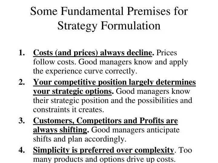
Some Fundamental Premises for Strategy Formulation. Costs (and prices) always decline . Prices follow costs. Good managers know and apply the experience curve correctly.

E N D
Some Fundamental Premises for Strategy Formulation • Costs (and prices) always decline. Prices follow costs. Good managers know and apply the experience curve correctly. • Your competitive position largely determines your strategic options. Good managers know their strategic position and the possibilities and constraints it creates. • Customers, Competitors and Profits are always shifting. Good managers anticipate shifts and plan accordingly. • Simplicity is preferred over complexity. Too many products and options drive up costs.
The Benefits in Low costs Original Price New Price Cost 2 Company 2 New Margins Cost1 Company 1 Note that because of Co. 1’s lower costs, the drop in price affects Co. 1’s margins proportionately less than co.2’s (approximately 1/3 vs. ½ in diagrams).
High R.O.I Low Low Mkt. Share High Assumed causal relationships: High Market Share Causes High Accumulated Volumes of Production Causes Low per Unit Costs High Profits
10th unit = $100 Then 20th unit = $100 * .85 =$85 Then 40th unit = $85*.85 = $72.25 An 85% Experience Curve 120 110 A 100 Deflated Direct cost per Unit 90 B 80 C D 70 60 E 50 40 30 20 10 0 10 20 30 40 50 60 70 80 90 100 120 130 Accumulated Vol. Of Production (units)
The Learning Effect n Y = 2X Where y = the no.(cost) of direct labor hrs required to produce the xth unit a = the no.(cost) of direct labor hrs required to produce the first unit x = the cumulative unit no. n = the learning index = (log 0)/(log 2) 0 = the learning rate 1-0 = the progress ration 1.0 Direct Labor hrs/unit 10 % progress (0 =90) .1 20% progress(0=80%) .01 30% progress (0=70%) .001 10 1000 100 Cumulative units as plotted logarithmetrically
Paper Airplane Exercise Results on Linear Scale $5 Trial 1 4 Cost Per Airplane 3 Trial 2 2 Trial 3 1 9 6 12 0 3 Accumulative Experience (Number of Planes)
Paper Airplane Exercise Results on Log Scale $10 Slope = 74% R2 = 1.00 5 Trial 1 Cost Per Airplane Trial 2 Trial 3 2 1 5 10 15 0 2 Accumulative Experience (Number of Planes)
Example Using Traditional Linear Programming Maximize : TT = $33X1 + $39X2 +$59X3 Subject to: 10X1 +15X2 +12X3 < or = 14,400 labor hours Production Constrain 24X1 + 20X2 + 14X3 < 0R = 5,900 machine hours Here, our optimal solution would be to produce: 0 units of X1 0 units of X2 361 units of X3 With resulting contribution margin of: $59 (361) = $21,299 This would yield optimal solution if there are no learning effects present. If, however, workers learn, machines are used more efficiently, and materials usage is optimized, then we would have to modify our linear programming formula. For example, that learning occurs such that there is a 90% experience curve effect. Then, if we were to only produce X the constraints on production change: Using logs 12X3.848 < or = 14,400 labor hrs 14X3.848 < or = 5,920 machine time We obtain 36X 3.848 < or = 13,026 materials Yields an optimal solution of $59 (1,040X) = $61,360
Experience Curve for Price of Brokerage Services 30¢ Slope = 64% R2 = 099 1990 20 EXECUTION REVENUE PER SHARE TRADED (intuitional: 1996 Dollars 10 5 2003 3 300 500 5,000 10,000B 1,000 2,000 CUMMULATIVE SHARES TRADED
3% Off $0.97 Full Price $1.00 Profit 8.1% Costs: 91.9% Profit 5.1% Costs: 91.9% The Perils of a Price Cut • An innocent little 3% price cut by the average S&P 1000 knocks the profits down from 8.1% to 5.1% or a whopping 37%
Incremental Breakeven Analysis Δ q = Δp – (1-cm) Δ c cm- Δp + (1-cm) Δc Definitions: Δq---the breakeven sales increase in percentage; Δp---the magnitude of a price cut; Cm---the contribution margin in percentage (before the price cut); Δc---the reduction in marginal costs in percentage due to the price cut.
Incremental Breakeven Analysis Δ q = Δp – (1-cm) Δ c cm- Δp + (1-cm) Δc Definitions: using Galanz example Δq---the breakeven sales increase in percentage = 90.5%; Δp---the magnitude of a price cut = 20%; Cm---the contribution margin in percentage (before the price cut) or (price – marginal cost) = 40%; Δc---the reduction in marginal costs in percentage due to the price cut = 35%
Circumstances for a Price War • High growth markets • Heterogeneous firms with a wide distribution of cost efficiencies • New technologies with significant scale economies
Source of the Experience Effect • Labor efficiency • New processes and improved methods • Product redesign • Product standardization • Scale effect • Substitution in the product
Practical Considerations • Cost-time relationship • High-volume effect • Shared experience • Product Definition • Cost data • Marginal vs. average cost • Inflation • Planning horizon • External influences • Market instability
Steps in A Typical Value-Added Chain: Product R & D Process R & D Purchasing of Raw Materials Transportation of Raw Materials Mfg. Of Parts and Components Assembly Testing and Quality Control Marketing Sales to intermediaries Wholesale Distribution Retailing After sales Service
The Generic Value Chain Firm Infrastructure Human Resource Management Support Activities Technology Development Procurement Operations Marketing & Sales Inbound Logistics Outbound Logistics Service Margin Upstream Value Activities Downstream Value Activities Primary Activities Economies of Scale Dominate Economies of Scope Dominate
Effects of accumulated experience over the cost accrued in different stages of value added Purchasing and Mfg of parts & Components R& D Subassembly Marketing Distribution Retail Deflated direct cost per unit 95% 75% 70% 90% 85% 95% Accumulated Volume of production in each stage (in units) R& D Manufacture Assembly Marketing Distribution Retail 2% 20% 15% 30% 25% 8% Accumulated Costs in each stage
Mkt. Leader is A w/rel. mkt share of 4 to 1 over B. Conceptualize value-added in 2 stage mfg and dist. In mfg. Stage A has the 4 to 1 advantage over B but in dist. Stage B has 3 to 1 advantage in terms of mkt share, because this is just one of many others that share the same system of dist. If we assume that experience in both stages has the same impact over costs, and that each stage contributes half the final value of the product, we could use a normalized mkt share to determine the relative standing of the 2 firms in the business. Two firm ex. W/value added as manufacturing and distribution for firm A: Market Share = (Mfg. Share x Mfg. Value-Added) + (Distribution Market Share x Distribution Value-Added) = [(4 to 1 or 4/5)] + [(1 to 3 or I/4) x (0.5)] = 0.525 Similarly for firm B Market Share = 0.475 The relative market share of firm A over firm B using this weighted measure of experience in only 0.525/0.475 = 1.10 times, for smaller than the observed to 4 to 1 product ratio in the final market.
Gillette Razor Blades Industry Life cycle Sales Business Life Cycle Waves of Product life cycle Wave of Profit Stainless Steel Blue Blades Super Chromium Platinum plus Time
Location of product in: a less developed country a newly industrialized country a fully developed country Sales $ Time
Costs – Sales – Profit Relationships by Stages of life Cycle Total Sales Costs/Unit Price/Unit Profit loss Loss Maturity Rapid Growth Introduction Decline
Growth – Share Matrix 22% 20 % Mkt. Growth Rate 18% 16% 14% 12% 10% 8% 6% 4% 2% 10X 4X 1.5X 1.0X 0.5X 0.1X Relative Competitor Position
Industry growth (Total Ind. Sales 2009) – (Total Ind. Sales 2008) Rate (2009) = Total Ind. Sales 2008 Relative Industry Your business unit’s sales Share = Leading competitor’s sales Circle Size = Your business unit’s sales Total corp. sales 4 ways to separate high-low growth • Avg. industry growth –single industry • Overall economic growth – multiple industry • Weighted average growth • Corporate growth target
Ideal Movement of Products and cash in the Portfolio Market Growth Relative Competitive Position = Cash Movement = Product movement
Using the Matrix to Guide Strategy The process consists of 3 steps: • Developing matrices for ones’ own firm. • Developing matrices for ones’ competitors. • Making strategic comparisons and generating strategies. Each step may be further subdivided: 1.a. Identify the products and the business sectors. 1.b. Selecting and ranking the criteria for assessing the Bus. Pos. and Ind. Attractiveness. 1.c. Gathering the data. 1.d. Quantifying each product’s position. 1.e. Drawing the matrices; past, present, and future. 1.f Assessing the implications of each product’s position in the matrix.