Download
1 / 52
520 likes | 679 Vues
C hapter 5. Mean-variance frontier and beta representations. Main contents. Expected return-Beta representation Mean-variance frontier: Intuition and Lagrangian characterization An orthogonal characterization of mean-variance frontier Spanning the mean-variance frontier

E N D
Main contents • Expected return-Beta representation • Mean-variance frontier: Intuition and Lagrangian characterization • An orthogonal characterization of mean-variance frontier • Spanning the mean-variance frontier • A compilation of properties of • Mean-variance frontiers for m: H-J bounds
Remark(1) • In (1), the intercept is the same for all assets. • In (2), the intercept is different for different asset. • In fact, (2) is the first step to estimate (1). • One way to estimate the free parameters is to run a cross sectional regression based on estimation of beta is the pricing errors
Remark(2) • The point of beta model is to explain the variation in average returns across assets. • The betas are explanatory variables,which vary asset by asset. • The alpha and lamda are the intercept and slope in the cross sectional estimation. • Beta is called as risk exposure amount, lamda is the risk price. • Betas cannot be asset specific or firm specific.
Some common special cases • If there is risk free rate, • If there is no risk-free rate, then alpha is called (expected)zero-beta rate. • If using excess returns as factors, (3) • Remark: the beta in (3) is different from (1) and (2). • If the factors are excess returns, since each factor has beta of one on itself and zero on all the other factors. Then, • 这个模型只研究风险溢酬,与无风险利率无关
5.2 Mean-Variance Frontier: Intuition and Lagrangian Characterization
Mean-variance frontier • Definition: mean-variance frontier of a given set of assets is the boundary of the set of means and variances of returns on all portfolios of the given assets. • Characterization: for a given mean return, the variance is minimum.
With or without risk free rate tangency risk asset frontier original assets mean-variance frontier
When does the mean-variance exist? • Theorem: So long as the variance-covariance matrix of returns is non singular, there is mean-variance frontier. • Intuition Proof: • If there are two assets which are totally correlated and have different mean return, this is the violation of law of one price. The law of one price implies the existence of mean variance frontier as well as a discount factor.
Mathematical method: Lagrangian approach • Problem: • Lagrangian function:
Mathematical method: Lagrangian approach(2) • First order condition: • If the covariance matrix is non singular, the inverse matrix exists, and
Mathematical method: Lagrangian approach(3) • In the end, we can get
Remark • By minimizing var(Rp) over u,giving
5.3 An orthogonal characterization of mean variance frontier
Introduction • Method: geometric methods. • Characterization: rather than write portfolios as combination of basis assets, and pose and solve the minimization problem, we describe the return by a three-way orthogonal decomposition, the mean variance frontier then pops out easily without any algebra.
Theorem: • Every return Ri can be expressed as: • Where is a number, and ni is an excess return with the property E(ni)=0. • The three components are orthogonal,
Proof: Geometric method R=space of return (p=1) Rf=R*+RfRe* R*+wiRe* R* 1 等预期超额收益率线 0 Re* E=1 E=2 E=0 Re =space of excess return (p=0) NOTE:1、支付空间为三维的。2、横的平面必须与竖的平面垂直。3、如果有无风险证券,则竖的平面过1点,否则不过,此时图上的1就是1在支付空间的投影。
Proof: Algebraic approach • Directly from definition, we can get
Remark • The minimum second moment return is not the minimum variance return.(why?) E(R) R*+wiRe* Ri R*
Spanning the mean variance frontier • With any two portfolios on the frontier. we can span the mean-variance frontier. • Consider
Properties(1) • Proof:
Properties(2) • Proof:
Properties(3) • can be used in pricing. • Proof: • For returns,
Properties(4) • If a risk-free rate is traded, • If not, this gives a “zero-beta rate” interpretation.
Properties(5) • has the same first and second moment. • Proof: • Then
Properties(6) • If there is risk free rate, • Proof:
If there is no risk free rate • Then the 1 vector can not exist in payoff space since it is risk free. Then we can only use
Properties(7) • Since • We can get
Properties(8) • Following the definition of projection, we can get • If there is risk free rate,we can also get it by:
5.6 Mean-Variance Frontiers for Discount Factors: The Hansen-Jagannathan Bounds
Mean-variance frontier for m: H-J bounds • The relationship between the Sharpe ratio of an excess return and volatility of discount factor. • If there is risk free rate,
Remark • We need very volatile discount factors with a mean near one to price the stock returns.
The behavior of Hansen and Jagannathan bounds • For any hypothetical risk free rate, the highest Sharpe ratio is the tangency portfolio. • Note: there are two tangency portfolios, the higher absolute Sharpe ratio portfolio is selected. • If risk free rate is less than the minimum variance mean return, the upper tangency line is selected, and the slope increases with the declination of risk free rate, which is equivalent to the increase of E(m).
The behavior of Hansen and Jagannathan bounds • On the other hand, if the risk free rate is larger than the minimum variance mean return, the lower tangency line is selected,and the slope decreases with the declination of risk free rate, which is equivalent to the increase of E(m). • In all, when 1/E(m) is less than the minimum variance mean return, the H-J bound is the decreasing function of E(m). When 1/E(m) is larger than the minimum variance mean return, the H-J bound is an increasing function.
Graphic construction E(R) 1/E(m) E(m)
Duality • A duality between discount factor volatility and Sharpe ratios.
Explicit calculation • A representation of the set of discount factors is • Proof:
Graphic Decomposition of discount factor X=payoff space M=space of discount factors x*+we* x* Proj(1lX) 1 0 e* E()=1 E()=2 E()=0 E =space of m-x* NOTE:横的平面必须与竖的平面垂直。
Special case • If unit payoff is in payoff space, • The frontier and bound are just • And • This is exactly like the case of state preference neutrality for return mean-variance frontiers, in which the frontier reduces to the single point R*.
Mathematical construction • We have got