Download

1 / 73
730 likes | 878 Vues
Stochastic Nonparametric Framework for Basin Wide Streamflow and Salinity Modeling Application to Colorado River basin Study Progress Meeting James R. Prairie August 17, 2006. Recent progress. Stochastic streamflow conditioned on Paleo Flow Non homogenous Markov Chain with Kernel Smoothing

E N D
Stochastic Nonparametric Framework for Basin Wide Streamflow and Salinity Modeling Application to Colorado River basin Study Progress Meeting James R. Prairie August 17, 2006
Recent progress Stochastic streamflow conditioned on Paleo Flow Non homogenous Markov Chain with Kernel Smoothing Estimate lag-1 two state transition probabilities for each year using a Kernel Estimator Generate Flow State Conditionally Generate flow magnitude Colorado River Basin Wide flow simulation Modify the nonparametric space-time disagg approach to generate monthly flows at all the 29 stations simultaneously Flow simulation using Paleo recontructions
Masters Research Single site Modified K-NN streamflow generator Climate Analysis Nonparametric Natural Salt Model Stochastic Nonparametric Technique for Space-Time Disaggregation Basin Wide Natural Salt Model Incorporate Paleoclimate Information Streamflow conditioned on “Flow States” from Paleo reconstructions Policy Analysis Impacts of drought Hydrology Water quality
Generate system state Generate flow conditionally (K-NN resampling) Proposed Methods Block bootstrap resampling of Paleo flows Nonhomogeneous Markov model Markov Chain on a 30-yr window Nonhomogeneous Markov model with smoothing or or
Datasets • Paleo reconstruction from Woodhouse et al. 2006 • Water years 1490-1997 • Observed natural flow from Reclamation • Water years 1906-2003
Addressing previous issues • Determined order of the Markov model • used AIC (Gates and Tong, 1976) • Indicated order 0 (or 1) - we used order 1 • Subjective block length and window for estimating the Markov Chain Transition Probabilities • Nonhomogeneous Markov Chain with Kernel Smoothing alleviates this problem (Rajagopalan et al., 1996)
Nonhomogenous Markov model with Kernel smoothing (Rajagopalan et al., 1996) • 2 state, lag 1 model chosen • ‘wet (1)’ if flow above annual median of observed record; ‘dry (0)’ otherwise. • AIC used for order selection (order 1 chosen) • TP for each year are obtained using the Kernel Estimator
window = 2h +1 Discrete kernal function h
Nonhomogenous Markov model with Kernel smoothing (Rajagopalan et al., 1996) K(x) is a discrete quadratic Kernel (or weight function) • ‘h’ is the smoothing window obtained objectively using Least Square Cross Validation
Window length chosen with LSCV 3 states
Simulation Algorithm • Determine planning horizon We chose 98yrs (same length as observational record) • Select 98 year block at random For example 1701-1798 • Generate flow states for each year of the resampled block using their respective TPMs estimated earlier NHMC • Generate flow magnitudes for each year by resampling observed flow using a conditional K-NN method • Repeat steps 2 through 4 to obtain as many required simulations
Advantages over block resampling • No need for a subjective window length • i.e., 30 year window was used to estimate the TP • Obviates the need for additional sub-lengths within the planning horizon • i.e., earlier 3 30-yr blocks were resampled • Fully Objective in estimating the TPMs for each year
ISM 98 simulations 98 year length No Conditioning
ISM 98 simulations 60 year length No Conditioning
Paleo Conditioned • NHMC with smoothing • 500 simulations • 98 year length
Paleo Conditioned • NHMC with smoothing • 500 simulations • 60 year length
Drought and Surplus Statistics Surplus Length Surplus volume flow Drought Length Threshold (e.g., mean) time Drought Deficit
No Conditioning • ISM • 98 simulations • 98 year length
Paleo Conditioned • NHMC with smoothing • 2 states • 500 simulations • 98 year length
Paleo Conditioned • Markov chain length 31 years • 2 states • 500 simulations • 98 year length
Sequent Peak Algorithm • Determine required Storage Capacity (Sc) at various demand levels given specified inflows. • Evaluate risk of not meeting the required Sc y = inflow time series (2x) d = demand level S = storage S’0= 0 if positive otherwise
No Conditioning • ISM • 98 simulations • 98 year length 60
No Conditioning • Traditional KNN • 98 simulations • 98 year length 60
Paleo Conditioned • NHMC with smoothing • 500 simulations • 98 year length 60
Paleo Conditioned • PDF of 16.5 boxplot • Red hatch represents risk of not meeting 16.5 demand at a 60 MAF storage capacity
Paleo Conditioned • PDF of 16.5 boxplot
60 Paleo Conditioned • NHMC with smoothing • 500 simulations • 98 year length
Paleo Conditioned • PDF of 13.5 boxplot • Red hatch represents risk of not meeting 13.5 demand at a 60 MAF storage capacity
Paleo Conditioned • CDF of 13.5 boxplot
if positive if positive otherwise otherwise Storage Capacity – Firm Yield function • What is the maximum yield (Y) given a specific storage capacity (K) and flow sequence (Qt)? • Mathematically this can be answered with optimization Maximize Y Subject to:
Paleo Conditioned • NHMC with smoothing • 500 simulations • 98 year length
Basic Statistics • Preserved for observed data • Note max and min constrained in observed
Conclusions • Combines strength of • Reconstructed paleo streamflows: system state • Observed streamflows: flows magnitude • Develops a rich variety of streamflow sequences • Generates sequences not in the observed record • More variety: block bootstrap reconstructed streamflows • Most variety: nonhomogeneous Markov chain • TPM provide flexibility • Homogenous Markov chains • Nonhomogenous Markov chains • Use TPM to mimic climate signal (e.g., PDO) • Generate drier or wetter than average flows
Masters Research Single site Modified K-NN streamflow generator Climate Analysis Nonparametric Natural Salt Model Stochastic Nonparametric Technique for Space-Time Disaggregation Basin Wide Natural Salt Model Incorporate Paleoclimate Information Streamflow conditioned on Paleo states Streamflow conditioned with TPM Policy Analysis Impacts of drought Hydrology Water quality
Full basin disaggregation • Upper basin • 20 gauges (all above Lees Ferry, including Lees Ferry) • Annual total flow at Lees Ferry: modeled with modified K-NN • Disaggregate Lees Ferry: nonparametric disaggregation • Results in intervening monthly flows at CRSS nodes • Store the years resampled during the temporal disagg • Lower basin • 9 gauges (all gauges below Lees Ferry) • Select the month values for all sites in a given year based on the years stored above
Nonparametric disagg K-NN years applied
Advantages • Paleo-conditioned flows for entire basin • Upper Basin • Generate both annual and monthly flows not previously observed • Produces 92% of annual flows above Imperial Dam • Faithfully reproduces PDF and CDF for both intervening and total flows • Lower Basin • Produces 8% of annual flows above Imperial Dam • Preserves intermittent properties of tributaries • Faithfully reproduces all statistics • Easily incorporate reconstructions at Lees Ferry
Disadvantages • Upper Basin • Generates negative flows at rim gauges (7 out of 10 gauges) • Average of 1.5% negatives over all simulations (500 sims) • Is this important? • Two largest contributors only produce 2.2% • Can not capture cross over correlation (i.e. between last month of previous year and first month of the current year) • Improved in recent run (added a weighted resampling) • Can not generate large extremes beyond the observed • Annual flow model choice • Using Paleo flow magnitudes • Lower Basin • Can only generate observed flows
Lees Ferry • intervening
Lees Ferry • Total sum of intervening
Lees Ferry • Total sum of intervening • No first month current year with last month previous year weighting
Cisco • Total sum of intervening
Green River UT • Total sum of intervening
San Juan • Total sum of intervening
San Rafael • Total sum of intervening • 1.2% of flow above Lees • 6% negatives over 500 sims
Lower Basin • Resample observed months based on K-NN from Upper basin disaggregation
Abv Imperial Dam • Total sum of intervening
Little Colorado • Total sum of intervening