Download
1 / 14
140 likes | 264 Vues
Testing Differences in Population Variances. QSCI 381 – Lecture 42 (Larson and Farber, Sect 10.3). Recap – Testing Means. We used different tests when comparing means depending on whether we could assume that the population variances for the two populations were the same.

E N D
Testing Differences in Population Variances QSCI 381 – Lecture 42 (Larson and Farber, Sect 10.3)
Recap – Testing Means • We used different tests when comparing means depending on whether we could assume that the population variances for the two populations were the same. • Today we identify a test which can be used to test for differences between two population variances.
The F-distribution-I • Let and represent the sample variances of two populations. If both populations are normal and the population variances and are equal, then the sampling distribution of: is called an . F-distribution
The F-distribution-II • Properties of the F-distribution: • Positively skewed. • The curve is determined by the degrees of freedom for the numerator and that for the denominator. • The area under the curve is 1. • The mean value is approximately 1. • F-values are always larger than 0.
The Two-Sample F-test for Variances-I • A two-sample F-test is used to compare two population variances and when a sample is randomly selected from each population. The populations must be independent and normally distributed. The test statistic is: • where and represent the sample variances with . The degrees of freedom for the numerator is d.f.N=n1-1 and the degrees of freedom for the denominator is d.f.D=n2-1.
The Two-Sample F-test for Variances-II(Finding the rejection region for the test) • Specify the level of significance . • Determine the degrees of freedom for the numerator, d.f.N. • Determine the degrees of freedom for the denominator, d.f.D. • Determine whether this a one-tailed or a two-tailed test. • One-tailed – look up the F-table for d.f.N and d.f.D. • Two-tailed – look up the /2 F-table for d.f.N and d.f.D.
The Two-Sample F-test for Variances-III(Finding the rejection region for the test) One-tailed Two-tailed F0=2.901 F0=3.576 In EXCEL: FINV(prob,dfN,dfD) d.f.N=5; d.f.D=15; =0.05
Example-A-I • We sample two populations. The sample variances for the two populations are 9.622 (n1=46) and 10.352 (n2=51). Test the claim that the two variances are equal (=0.1). • H0: ; Ha: • Determine the critical value and the rejection region. • This is a two-tailed test. • We reverse the order of samples 1 and 2 so that . Therefore d.f.N=50; d.f.N=45. • The critical value is F(0.05,50,45) = 1.626.
Example-A-II • The test statistic is: • We fail to reject the null hypothesis
30 fish are sampled from a Marine Reserve and a fished area. Test the claim that the lengths in the Reserve are more variable than those in the fished area (assume =0.05). The data are: Example-B-I
Example-B-II • H0: ; Ha: • =0.05; d.f.N=29; d.f.D=29. This is a one-sided test so the rejection region is F>1.861 = FINV(0.05,29,29) • The test statistic is: • We reject the null hypothesis (the data provide support for the claim)
Confidence intervals for • When and are the variances of randomly selected, independent samples from normally distributed populations, a confidence interval for is: where FL is the left-tailed critical F-value and FR is the right-tailed critical F-value (based on probabilities of /2).
Confidence intervals for(Example-1) • Find a 95% confidence interval for for example A. • The lower and upper critical points for the F-distribution are computed: • FINV(0.975,50,45)=0.564 • FINV(0.025,50,45)=1.788
Confidence intervals for(Example-2) • The 95% confidence interval is given by: