Download
1 / 1
10 likes | 148 Vues
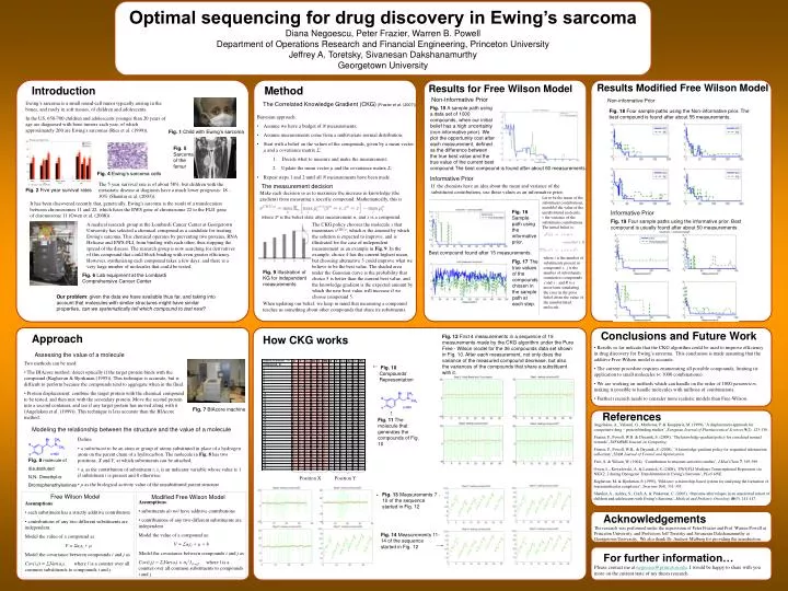
Optimal sequencing for drug discovery in Ewing’s sarcoma Diana Negoescu, Peter Frazier, Warren B. Powell Department of Operations Research and Financial Engineering, Princeton University Jeffrey A. Toretsky, Sivanesan Dakshanamurthy Georgetown University. Results Modified Free Wilson Model.

E N D
Optimal sequencing for drug discovery in Ewing’s sarcoma Diana Negoescu, Peter Frazier, Warren B. Powell Department of Operations Research and Financial Engineering, Princeton University Jeffrey A. Toretsky, Sivanesan Dakshanamurthy Georgetown University Results Modified Free Wilson Model Results for Free Wilson Model Introduction Ewing’s sarcoma is a small round-cell tumor typically arising in the bones, and rarely in soft tissues, of children and adolescents. In the US, 650-700 children and adolescents younger than 20 years of age are diagnosed with bone tumors each year, of which approximately 200 are Ewing's sarcomas (Ries et al. (1999)). Method Non-Informative Prior Non-informative Prior The Correlated Knowledge Gradient (CKG) (Frazier et al. (2007)) Fig. 15 A sample path using a data set of 1000 compounds, when our initial belief has a high uncertainty (non-informative prior). We plot the opportunity cost after each measurement, defined as the difference between the true best value and the true value of the current best compound. Fig. 18 Four sample paths using the Non-informative prior. The best compound is found after about 55 measurements. • Bayesian approach: • Assume we have a budget of N measurements; • Assume measurements come from a multivariate normal distribution; • Start with a belief on the values of the compounds, given by a mean vector μ and a covariance matrix Σ; • Decide what to measure and make the measurement; • 2. Update the mean vectorμ and the covariance matrix Σ; • Repeat steps 1 and 2 until all N measurements have been made. Fig. 1 Child with Ewing’s sarcoma Fig. 5 Sarcoma of the femur The best compound is found after about 60 measurements. Fig. 4 Ewing’s sarcoma cells Informative Prior The 5 year survival rate is of about 58%, but children with the metastatic disease at diagnosis have a much lower prognosis: 18 – 30% (Shankar et al. (2003)). The measurement decision If the chemists have an idea about the mean and variance of the substituent contributions, use these values as an informative prior. Fig. 2 Five year survival rates Make each decision so as to maximize the increase in knowledge (the gradient) from measuring a specific compound. Mathematically, this is Let m be the mean of the substituent contributions, mainMol the value of the unsubstituted molecule, v the variance of the substituent contributions. The initial belief is: It has been discovered recently that, genetically, Ewing's sarcoma is the result of a translocation between chromosomes 11 and 22, which fuses the EWS gene of chromosome 22 to the FLI1 gene of chromosome 11 (Owen et al. (2008)). Fig. 16 Sample path using the informative prior. Informative Prior where Snis the belief state after measurement n, and x is a compound. Fig. 19 Four sample paths using the informative prior. Best compound is usually found after about 50 measurements. A medical research group at the Lombardi Cancer Center at Georgetown University has selected a chemical compound as a candidate for treating Ewing's sarcoma. This chemical operates by preventing two proteins, RNA Helicase and EWS-FLI, from binding with each other, thus stopping the spread of the disease. The research group is now searching for derivatives of this compound that could block binding with even greater efficiency. However, synthesizing each compound takes a few days, and there is a very large number of molecules that could be tested. The CKG policy chooses the molecule x that maximizes νCKG,n, which is the amount by which the solution is expected to improve, and is illustrated for the case of independent measurement as an example in Fig. 9. In the example, choice 4 has the current highest mean, but choosing alternative 5 could improve what we believe to be the best value. The shaded area under the Gaussian curve is the probability that choice 5 is better than the current best value, and the knowledge gradient is the expected amount by which the new best value will increase if we choose compound 5. Best compound found after 15 measurements. where i is the number of substituents present in compound x, j is the number of substituents common to compounds x and x’, and R is a noise term simulating the error in the prior belief about the value of the unsubstituted molecule. Fig. 17 The true values of the compounds chosen in the sample path at each step. Fig. 9 Illustration of KG for independent measurements Fig.6 Lab equipment at the Lombardi Comprehensive Cancer Center Our problem: given the data we have available thus far, and taking into account that molecules with similar structures might have similar properties, can we systematically tell which compound to test next? When updating our belief, we keep in mind that measuring a compound teaches us something about other compounds that share its substituents. Conclusions and Future Work Approach How CKG works Fig. 12 First 4 measurements in a sequence of 19 measurements made by the CKG algorithm under the Pure Free - Wilson model for the 36 compounds data set shown in Fig. 10. After each measurement, not only does the variance of the measured compound decrease, but also the variances of the compounds that share a substituent with it. • Results so far indicate that the CKG algorithm could be used to improve efficiency in drug discovery for Ewing’s sarcoma. This conclusion is made assuming that the additive Free-Wilson model is accurate. • The current procedure requires enumerating all possible compounds, limiting its application to small molecules (< 1000 combinations). • We are working on methods which can handle on the order of 1000 parameters, making it possible to handle molecules with millions of combinations. • Further research needs to consider more realistic models than Free-Wilson. Assessing the value of a molecule • Two methods can be used: • The BIAcore method: detect optically if the target protein binds with the compound (Raghavan & Bjorkman (1995)). This technique is accurate, but is difficult to perform because the compounds tend to aggregate when in the fluid. • Protein displacement: combine the target protein with the chemical compound to be tested, and then mix with the secondary protein. Move the second protein into a second container, and see if any target protein has moved along with it (Angelakou et al. (1999)). This technique is less accurate than the BIAcore method. Fig. 10 Compounds’ Representation Fig. 7 BIAcore machine References Fig. 11 The molecule that generates the compounds of Fig. 10 • Angelakou, A., Valsami, G., Macheras, P. & Koupparis, M. (1999), ‘A displacement approach for competitive drug – protein binding studies’, European Journal of Pharmaceutical Sciences9(2), 123-130. • Frazier, P., Powell, W.B. & Dayanik, S. (2009), ‘The knowledge-gradient policy for correlated normal rewards’, INFORMS Journal on Computing. • Frazier, P., Powell, W.B., & Dayanik, S. (2008), ‘A knowledge-gradient policy for sequential information collection’, SIAM Journal of Control and Optimization. • Free, S. & Wilson, W. (1964), ‘Contribution to structure-activities studies’, J Med Chem7, 395-399. • Owen, L., Kowalewski, A. & Lessnick, S. (2008), ‘EWS/FLI Mediates Transcriptional Repression via NKX2. 2 during Oncogenic Transformation in Ewing’s Sarcoma’, PLoS ONE. • Raghavan, M. & Bjorkman, P. (1995), ‘BIAcore: a microchip-based system for analyzing the formation of macromolecular complexes’, Structure3(4), 331-333. • Shankar, A., Ashley, S., Craft, A. & Pinkerton, C. (2003), ‘Outcome after relapse in an unselected cohort of children and adolescents with Ewing’s Sarcoma’, Medical and Pediatric Oncology40(3), 141-147. Modeling the relationship between the structure and the value of a molecule • Define • a substituent to be an atom or group of atoms substituted in place of a hydrogen atom on the parent chain of a hydrocarbon. The molecule in Fig. 8 has two positions, X and Y, at which substituents can be attached; • ai as the contribution of substituent i; si is an indicator variable whose value is 1 if substituent i is present and 0 otherwise; • μ as the biological activity value of the unsubstituted parent structure. Fig. 8molecule of disubstituted N,N- Dimethyl-α- Bromophenethylamines Fig. 13 Measurements 7 -10 of the sequence started in Fig. 12 Free Wilson Model Modified Free Wilson Model • Assumptions: • substituents do not have additive contributions • contributions of any two different substituents are independent. • Model the value of a compound as: • V = Σaisi + μ + b • Model the covariance between compounds i and j as • Cov(i,j) = ΣlVar(ai) + σb21{i=j}, where l is a counterover all common substituents to compounds i and j. • Assumptions: • each substituent has a strictly additive contribution • contributions of any two different substituents are independent. • Model the value of a compound as • V = Σaisi + μ • Model the covariance between compounds i and j as • Cov(i,j) = ΣlVar(ai), where l is a counter over all common substituents to compounds i and j. Acknowledgements The research was performed under the supervision of Peter Frazier and Prof. Warren Powell at Princeton University, and Professors Jeff Toretsky and Sivanesan Dakshanamurthy at Georgetown University. We also thank Dr. Andrew Mulberg for providing the introduction. Fig. 14 Measurements 11-14 of the sequence started in Fig. 12 For further information… Please contact me at negoescu@princeton.edu. I would be happy to share with you more on the current state of my thesis research.