Download
1 / 14
140 likes | 235 Vues
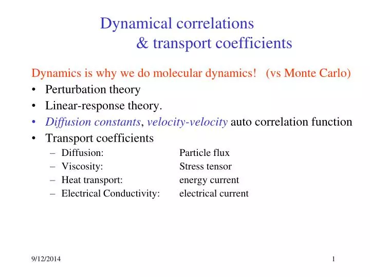
Dynamical correlations & transport coefficients. Dynamics is why we do molecular dynamics! (vs Monte Carlo) Perturbation theory Linear-response theory. Diffusion constants , velocity-velocity auto correlation function Transport coefficients Diffusion: Particle flux

E N D
Dynamical correlations & transport coefficients Dynamics is why we do molecular dynamics! (vs Monte Carlo) • Perturbation theory • Linear-response theory. • Diffusion constants, velocity-velocity auto correlation function • Transport coefficients • Diffusion: Particle flux • Viscosity: Stress tensor • Heat transport: energy current • Electrical Conductivity: electrical current
Static Perturbation theory Consider a perturbation by A(R). Change is distribution is: Expand in powers of : F() = F(0)+ <A>0 –2[<A2>0 –<A>02 ]/2 + … For a property B(R): B() = B(0) – [<AB>0 –<A>0 <B>0 ] + … Example let A=B=k, then: The structure factors gives the static response to a “density field” as measured by neutron and X-ray scattering (applied nuclear or electric field).
Dynamical Correlation Functions • If system is ergodic, ensemble average equals time average and we can average over t0. • Decorrelation at large times: • Autocorrelation function B=A*. Fourier transform:
Dynamical Properties • Fluctuation-Dissipation theorem: • We calculate the lhs average in equilibrium (no external perturbation). • [A e-iwt ] is a perturbation and [(w) e-iwt] is the response of B. • Fluctuations we “see” in equilibrium are equivalent to how a non-equilibrium system approaches equilibrium. (Onsager regression hypothesis; 1930 Nobel prize) • Density-Density response function is S(k,w). It can be measured by scattering and is sensitive to collective motions.
Linear Response in quantum mechanics • Reduces to classical formula when h=0
Transport coefficients • Define as the response of the system to some dynamical or long-term perturbation, e.g., velocity-velocity • Take zero frequency limit: • Kubo form: integral of time (auto-) correlation function. perturbation response
Transport Coefficients: examples These can also be evaluated with non-equilibrium simulations. • Impose a shear, heat or current flow • Initial difference in particle numbers Need to use thermostats to have a steady-statesimulation, otherwise energy (temperature) is not constant. • Diffusion: Particle flux • Viscosity: Stress tensor • Heat transport: energy current • Electrical Conductivity: electrical current J(t)=total electric current
Diffusion Constant • Defined by Fick’s law and controls how systems mix Linear response + Conservation of mass Einstein relation (no PBC!) Kubo formula • Use “unwound” positions to get equivalence between the 2 forms.
Consider a mixture of identical particles Initial condition Later
Alder-Wainwright discovered long-time tails on the velocity autocorrelation function. The diffusion constant does not exist in 2D because of hydrodynamic effects. • Results from computer simulation have changed our picture of a liquid. Several types of motion are allowed. • Train effect--one particle pulls other particle along behind it. • Vortex effect- at very long time one needs to solve using hydrodynamics--this dominates the long-time behavior. • Hard sphere interactions are able to model this aspect of a liquid.
Density-Density response: a sound wave • Measured by scattering and is sensitive to collective motions. • Suppose we have a sound wave: • Peaks in S(k,w) at q and -q. • Damping of sound wave broadens the peaks. • Inelastic neutron scattering can measure microscopic collective modes.
Dynamical Structure Factor for Hard Spheres For V0=Nd3/√2, HS fluid for V/V0 = 1.6, kd=0.38 V/V0 = 1.6, kd=2.28 V/V0 = 3.0, kd=0.44 V/V0 = 10, kd=0.41 Freq. = kd/, = mean collision time Points: MD (Alley et al, 1983) Lines: Enskog theory
Some experimental data from neutron scattering Water liquid 3 helium