Download
1 / 20
200 likes | 345 Vues
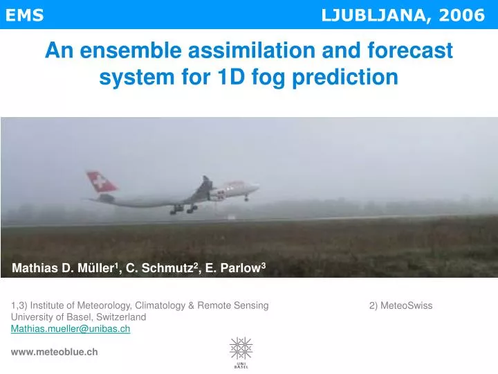
EMS LJUBLJANA, 2006. An ensemble assimilation and forecast system for 1D fog prediction. Mathias D. Müller 1 , C. Schmutz 2 , E. Parlow 3. 1,3) Institute of Meteorology, Climatology & Remote Sensing University of Basel, Switzerland Mathias.mueller@unibas.ch www.meteoblue.ch.

E N D
EMS LJUBLJANA, 2006 An ensemble assimilation and forecast system for 1D fog prediction Mathias D. Müller1, C. Schmutz2, E. Parlow3 1,3) Institute of Meteorology, Climatology & Remote Sensing University of Basel, Switzerland Mathias.mueller@unibas.ch www.meteoblue.ch 2) MeteoSwiss
1D fog modeling (COBEL-NOAH and PAFOG) Radiation land surface model Turbulence microphysics + initial (IC) and boundary conditions (BC)
Initial conditions • Initialization: • observations of • temperature & humidity • 3D model data: • aLMo, NMM-22, NMM-4, NMM-2 Data assimilation
Boundary conditions t 3D Valley fog Boundary conditions: From 3D models: aLMo, NMM-22, NMM-4, NMM-2 - Clouds - Advection of temperature & humidity
Initialization – Data assimilation error: „the magic“ background analysis observation 20 21.5 22 Temperatur B and R determine the relative importance analysis (x) observation (y) background (xb) 15 16 17 18 19 20 21 22 23 24 25 26 27 28 Temperature (°C)
Assimilation - B for 3 different 3D models (Winter) NMM-22 00 UTC NMM-4 1400 UTC NMM-4 00 UTC aLMo 00 UTC large model and time dependence
Initialization – Data assimilation (example) 21 hour forecast of NMM-2 28 Nov 2004 Zürich Airport
The ensemble forecast system Obser - vations 3D-Model runs 1D-models aLMo NMM-2 Fog forecast period B-matrices PAFOG variational assimilation COBEL-NOAH post-processing NMM-22 NMM-4 www.meteoblue.ch 3D - Forecast time Different IC and BC
Ensemble Forecast - Example 16 14 12 10 8 6 4 2 m rel. Hum. (%) 2 m Temperature (°C) 100 90 80 70 60 50 HEIGHT (m) fog INITIALIZED: 14 OCTOBER 2005 1500 UTC
Verification of the 1D ensemble forecast - ROC 1 10 40 60 HIT RATE no skill 60 60 10 fog: 0 1 FALSE ALARM RATE Fog – yes/no? ROC Fog (observation) = visibility < 1000 m Fog (model) = liquid water content > threshold has probability x
Verification of the 1D ensemble forecast - ROC Importance of Advection Sensitivity to humidity assimilation 03-11 UTC from 1 November 2004 until 30 April 2005
Hourly advection estimates (different 3D models) warm cool humid dry advection of cooler and drier air 03-11 UTC from 1 November 2004 until 30 April 2005
Verification of the 1D ensemble forecast - ROC 15:00 UTC 18:00 UTC - Initialisierungszeitpunkt - Multimodel 21:00 UTC 00:00 UTC PAFOG MODEL-ENSEMBLE COBEL-NOAH
Conclusions • 1D ensemble forecast has the potential to improve fog prediction at Zürich airport: • Advection (of cooler and drier air) is very important • Humidity assimilation with large uncertainty → more observations, humidity ensemble • COST-722 • MeteoSwiss 1D Thanks
3D simulations even more promising satellite Model
Assimilation – inkrementelle cost function (physical space) Write in incremental Form Introduce T and U transform to eliminate B from the cost function (Control variable space)
Assimilation – Error covariance Matrix NMC-Method (use 3D models):