Download
1 / 121
1.22k likes | 1.41k Vues
Topic 5 Instruction Scheduling. Superscalar (RISC) Processors. Function Units. Pipelined Fixed, Floating Branch etc. Register Bank. Canonical Instruction Set. Register Register Instructions (Single cycle).

E N D
Superscalar (RISC) Processors Function Units Pipelined Fixed, Floating Branch etc. Register Bank
Canonical Instruction Set • Register Register Instructions (Single cycle). • Special instructions for Load and Store to/from memory (multiple cycles). A few notable exceptions of course. Eg., Dec Alpha, HP-PA RISC, IBM Power & RS6K, Sun Sparc ...
Opportunity in Superscalars • High degree of Instruction Level Parallelism (ILP) via multiple (possibly) pipelined functional units (FUs). Essential to harness promised performance. • Clean simple model and Instruction Set makes compile-time optimizations feasible. • Therefore, performance advantages can be harnessed automatically
Example of Instruction Level Parallelism Processor components • 5 functional units: 2 fixed point units, 2 floating point units and 1 branch unit. • Pipeline depth: floating point unit is 2 deep, and the others are 1 deep. Peak rates: 7 instructions being processed simultaneously in each cycle
Instruction Scheduling: The Optimization Goal Given a source program P, schedule the instructions so as to minimize the overall execution time on the functional units in the target machine.
Cost Functions • Effectiveness of the Optimizations: How well can we optimize our objective function? Impact on running time of the compiled code determined by the completion time. • Efficiency of the optimization: How fast can we optimize? Impact on the time it takes to compile or cost for gaining the benefit of code with fast running time.
Impact of Control Flow Acyclic control flow is easier to deal with than cyclic control flow. Problems in dealing with cyclic flow: • A loop implicitly represent a large run-time program space compactly. • Not possible to open out the loops fully at compile-time. • Loop unrolling provides a partial solution. more...
Impact of Control Flow (Contd.) • Using the loop to optimize its dynamic behavior is a challenging problem. • Hard to optimize well without detailed knowledge of the range of the iteration. • In practice, profiling can offer limited help in estimating loop bounds.
Acyclic Instruction Scheduling • We will consider the case of acyclic control flow first. • The acyclic case itself has two parts: • The simpler case that we will consider first has no branching and corresponds to basic block of code, eg., loop bodies. • The more complicated case of scheduling programs with acyclic control flow with branching will be considered next.
The Core Case: Scheduling Basic Blocks Why are basic blocks easy? • All instructions specified as part of the input must be executed. • Allows deterministic modeling of the input. • No “branch probabilities” to contend with; makes problem space easy to optimize using classical methods.
Early RISC Processors Single FU with two stage pipeline: Logical (programmer’s view of: Berkeley RISC, IBM801, MIPS Register Bank
Instruction Execution Timing The 2-stage pipeline of the Functional Unit • The first stage performs Fetch/Decode/Execute for register-register operations (single cycle) and fetch/decode/initiate for Loads and Stores from memory (two cycles). more... Stage 1 Stage 2 1 Cycle 1 Cycle
Instruction Execution Timing • The second cycle is the memory latency to fetch/store the operand from/to memory. In reality, memory is cache and extra latencies result if there is a cache miss.
Parallelism Comes From the Following Fact While a load/store instruction is executing at the second pipeline stage, a new instruction can be initiated at the first stage.
Instruction Scheduling For previous example of RISC processors, Input:A basic block represented as a DAG • i2is a load instruction. • Latency of 1 on (i2,i4) means that i4 cannot start for one cycle after i2 completes. i2 0 1 Latency i1 i4 0 0 i3
Instruction Scheduling (Contd.) Two schedules for the above DAG with S2 as the desired sequence. Idle Cycle Due to Latency S1 i1 i3 i2 i4 S2 i1 i2 i3 i4
The General Instruction Scheduling Problem Input: DAG representing each basic block where: 1. Nodes encode unit execution time (single cycle) instructions. 2. Each node requires a definite class of FUs. 3. Additional pipeline delays encoded as latencies on the edges. 4. Number of FUs of each type in the target machine. more...
The General Instruction Scheduling Problem (Contd.) Feasible Schedule: A specification of a start time for each instruction such that the following constraints are obeyed: 1. Resource: Number of instructions of a given type of any time < corresponding number of FUs. 2. Precedence and Latency: For each predecessor j of an instruction i in the DAG, i is the started only cycles after j finishes where is the latency labeling the edge (j,i), Output: A schedule with the minimum overall completion time (makespan).
Drawing on Deterministic Scheduling Canonical Algorithm: 1. Assign a Rank (priority) to each instruction (or node). 2. Sort and build a priority list ℒ of the instructions in non-decreasing order of Rank. Nodes with smaller ranks occur either in this list.
Drawing on Deterministic Scheduling (Contd.) 3. Greedily list-scheduleℒ. Scan ℒ iteratively and on each scan, choose the largest number of “ready” instructions subject to resource (FU) constraints in list-order. An instruction is ready provided it has not been chosen earlier and all of its predecessors have been chosen and the appropriate latencies have elapsed.
The Value of Greedy List Scheduling Example: Consider the DAG shown below: Using the list ℒ = <i1, i2, i3, i4, i5> • Greedy scanning produces the steps of the schedule as follows: more...
The Value of Greedy List Scheduling (Contd.) 1. On the first scan: i1 which is the first step. 2. On the second and third scans and out of the list order, respectively i4 and i5 to correspond to steps two and three of the schedule. 3. On the fourth and fifth scans, i2 and i3 respectively scheduled in steps four and five.
Some Intuition • Greediness helps in making sure that idle cycles don’t remain if there are available instructions further “down stream.” • Ranks help prioritize nodes such that choices made early on favor instructions with greater enabling power, so that there is no unforced idle cycle.
How Good is Greedy? Approximation: For any pipeline depth k ≥ 1 and any number m of pipelines, 1 Sgreedy/Sopt ≤ (2 - ----- ). mk • For example, with one pipeline (m=1) and the latencies k grow as 2,3,4,…, the approximate schedule is guaranteed to have a completion time no more 66%, 75%, and 80% over the optimal completion time. • This theoretical guarantee shows that greedy scheduling is not bad, but the bounds are worst-case; practical experience tends to be much better. more...
How Good is Greedy? (Contd.) Running Time of Greedy List Scheduling: Linear in the size of the DAG. “Scheduling Time-Critical Instructions on RISC Machines,” K. Palem and B. Simons, ACM Transactions on Programming Languages and Systems, 632-658, Vol. 15, 1993.
Rank Functions 1. “Postpass Code Optimization of Pipelined Constraints”, J. Hennessey and T. Gross, ACM Transactions on Programming Languages andSystems, vol. 5, 422-448, 1983. 2. “Scheduling Expressions on a Pipelined Processor with a Maximal Delay of One Cycle,” D. Bernstein and I. Gertner, ACM Transactions on ProgrammingLanguages and Systems, vol. 11 no. 1, 57-66, Jan 1989.
Rank Functions (Contd.) 3. “Scheduling Time-Critical Instructions on RISC Machines,” K. Palem and B. Simons, ACM Transactions on Programming Languages andSystems, 632-658, vol. 15, 1993 Optimality: 2 and 3 produce optimal schedules for RISC processors such as the IBM 801, Berkeley RISC and so on.
An Example Rank Function The example DAG 1. Initially label all the nodes by the same value, say 2. Compute new labels from old starting with nodes at level zero (i4) and working towards higher levels: (a) All nodes at level zero get a rank of . more... i2 0 1 Latency i1 i4 0 0 i3
An Example Rank Function (Contd.) (b) For a node at level 1, construct a new label which is the concentration of all its successors connected by a latency 1 edge. Edgei2 toi4 in this case. (c) The empty symbol is associated with latency zero edges. Edges i3 toi4 for example.
An Example Rank Function (d) The result is that i2 and i3 respectively get new labels and hence ranks ’= > ’’ = . Note that ’= > ’’ = i.e., labels are drawn from a totally ordered alphabet. (e) Rank of i1 is the concentration of the ranks of its immediate successors i2 and i3 i.e., it is ’’’= ’|’’. 3. The resulting sorted list is (optimum) i1, i2, i3, i4.
The More General Case Scheduling Acyclic Control Flow Graphs
Significant Jump in Compilation Cost What is the problem when compared to basic-blocks? • Conditional and unconditional branching is permitted. • The problem being optimized is no longer deterministically and completely known at compile-time. • Depending on the sequence of branches taken, the problem structure of the graph being executed can vary • Impractical to optimize all possible combinations of branches and have a schedule for each case, since a sequence of k branches can lead to 2k possibilities -- a combinatorial explosion in cost of compiling.
Containing Compilation Cost A well known classical approach is to consider traces through the (acyclic) control flow graph. An example is presented in the next slide.
START BB-3 BB-1 BB-2 BB-4 BB-5 BB-6 A trace BB-1, BB-4, BB-6 BB-7 Branch Instruction STOP
Traces “Trace Scheduling: A Technique for Global Microcode Compaction,” J.A. Fisher, IEEE Transactions on Computers, Vol. C-30, 1981. Main Ideas: • Choose a program segment that has no cyclic dependences. • Choose one of the paths out of each branch that is encountered. more...
Traces (Contd.) • Use statistical knowledge based on (estimated) program behavior to bias the choices to favor the more frequently taken branches. • This information is gained through profiling the program or via static analysis. • The resulting sequence of basic blocks including the branch instructions is referred to as a trace.
Trace Scheduling High Level Algorithm: 1. Choose a (maximal) segment s of the program with acyclic control flow. The instructions in s have associated “frequencies” derived via statistical knowledge of the program’s behavior. 2. Construct a trace through s: (a) Start with the instruction in s, say i, with the highest frequency. more...
Trace Scheduling (Contd.) (b) Grow a path out from instruction i in both directions, choosing the path to the instruction with the higher frequency whenever there is Frequencies can be viewed as a way of prioritizing the path to choose and subsequently optimize. 3. Rank the instructions in using a rank function of choice. 4.Sort and construct a list ℒ of the instructions using the ranks as priorities. 5. Greedily list schedule and produce a schedule using the list ℒ as the priority list.
Significant Comments • We pretend as if the trace is always taken and executed and hence schedule it in steps 3-5 using the same framework as for a basic-block. • The important difference is that conditionals branches are there on the path, and moving code past these conditionals can lead to side-effects. • These side effects are not a problem in the case of basic-blocks since there, every instruction is executed all the time. • This is not true in the present more general case when an outgoing or incoming off-trace branch is taken however infrequently: we will study these issues next.
The Four Elementary but Significant Side-effects Consider a single instruction moving past a conditional branch: Branch Instruction Instruction being moved
The First Case • This code movement leads to the instruction executing sometimes when the instruction ought not to have: speculatively. more... If A is a DEF Live Off-trace False Dependence Edge Added A Off-trace Path
The First Case (Contd.) • If A is a write of the form a:= …, then, the variable (virtual register) a must not be live on the off-trace path. • In this case, an additional pseudo edge is added from the branch instruction to instruction A to prevent this motion.
The Second Case • Identical to previous case except the pseudo-dependence edge is from A to the join instruction whenever A is a “write” or a def. • A more general solution is to permit the code motion but undo the effect of the speculated definition by adding repair code An expensive proposition in terms of compilation cost. Edged added
The Third Case A • Instruction A will not be executed if the off-trace path is taken. • To avoid mistakes, it is replicated. more... Replicate A Off-trace Path
The Third Case (Contd.) • This is true in the case of read and write instructions. • Replication causes A to be executed independent of the path being taken to preserve the original semantics. • If (non-)liveliness information is available , replication can be done more conservatively.
The Fourth Case • Similar to Case 3 except for the direction of the replication as shown in the figure above. Off-trace Path Replicate A A
At a Conceptual Level: Two Situations • Speculations: Code that is executed “sometimes” when a branch is executed is now executed “always” due to code motion as in Cases 1 and 2. • Legal speculations wherein data-dependences are not violated. • Safe speculation wherein control-dependences on exceptions-causing instructions are not violated. more...