Download
1 / 17
190 likes | 218 Vues
Propagating Uncertainty In POMDP Value Iteration with Gaussian Process. Written by Eric Tuttle and Zoubin Ghahramani Presenter by Hui Li May 20, 2005. Outline: Framework of POMDP Framework of Gaussian Process Gaussian Process Value Iteration Results Conclusions. Framework of POMDP.

E N D
Propagating Uncertainty In POMDP Value Iteration with Gaussian Process Written by Eric Tuttle and Zoubin Ghahramani Presenter by Hui Li May 20, 2005
Outline: • Framework of POMDP • Framework of Gaussian Process • Gaussian Process Value Iteration • Results • Conclusions
Framework of POMDP The POMDP is defined by the tuple < S, A, T, R, ,O> • S is a finite set of states of the world. • A is a finite set of actions. • T: SA (S) is the state-transition function, the probability of an action changing the the world state from one to another,T(s, a, s’). • R: SA is the reward for the agent in a given world state after performing an action, R(s, a). is a finite set of observations. • O: SA () is the observation function, the probability of making a certain observation after performing a particular action, landing in state s’, O(s’, a, o).
WORLD Action Observation AGENT b SE POMDP agent can be decomposed into two parts: a state estimator (SE) and a policy (). o b a
The goal of a POMDP agent is to select actions which maximize its expected total sum of future rewards . • Two functions are most often used in reinforcement learning algorithms: • value function (function of state) Optimal value function: • Q function (function of state-action) Optimal value function:
The key assumption of POMDP is that the state is unknown, partially observable. We rely on the concept of a belief state, denoted b, to represent a probability distribution over states. The belief is a sufficient statistic for a given history:
After taking an action a and seeing an observation o, the agent updates its belief state using Bayes’ rule:
Bellman’s equations for POMDP are as follows: Bellman’s equations for value function Bellman’s equations for Q function
Framework of Gaussian Process regression A Gaussian process regressor defines a distribution over possible functions that could fit the data. In particular, the distribution of a function y(x) is a Gaussian process if the probability density p(y(x1), y(x2), …, y(xN)) for any finite set of points {x1,…, xN} is a multivariate Gaussian.
Assume we have a Gaussian process with mean 0 and covariance function K(xi, xj). Suppose we have observed a set of training points and target function values D = {(xn,tn), n = 1,…, N}. ~ N(0, ), a Gaussian noise. Then C = + K. With a new data x’, we have
One general choice of covariance function is: With W a diagonal matrix. : expected amplitude of the function : a bias term that accommodates non-zero-mean functions. Using maximum likelihood or MAP methods, the parameters of the covariance function can be tuned.
Gaussian Process Value Iteration Q function: Model each of the action value functions Q( ,a) as a Gaussian process. According to the definition of the Gaussian process, Qt-1( ,a) is a multivariate normal distribution with mean a,boand covariance a,bo. The major problem in computing the distribution Qt(b,a) is the max operator.
Two approximate ways for dealing with the max operator: 1. Approximate the max operator as simply passing through the random variable with the highest mean. Where
2. Take into account the effects of the max operator, but ignore correlations among the function values. If q1 and q2 are independent with distributions: Then first two moments of variable q = max( q1, q2) are given: Where is the cdf and is the pdf for a zero mean, unit variance normal. And q can be approximate using a Gaussian distribution.
Based on that, we can use a Gaussian distribution to approximate Both methods produce a Gaussian approximation for the max of a set of normally distributed vectors. And since Qta is related to Qt-1* by a linear transformation , we have:
Conclusions • In this paper, authors presented an algorithms – Gaussian processes for approximate value iteration in POMDPs. • The results using GP are comparable to that of the classical methods.