Download
1 / 33
330 likes | 543 Vues
Introduction to Neural Networks. John Paxton Montana State University Summer 2003. Chapter 7: A Sampler Of Other Neural Nets. Optimization Problems Common Extensions Adaptive Architectures Neocognitron. I. Optimization Problems. Travelling Salesperson Problem. Map coloring.

E N D
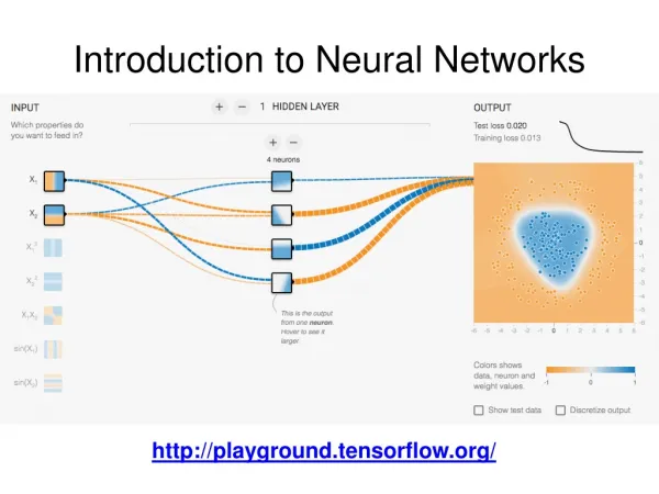
Introduction to Neural Networks John Paxton Montana State University Summer 2003
Chapter 7: A Sampler Of Other Neural Nets • Optimization Problems • Common Extensions • Adaptive Architectures • Neocognitron
I. Optimization Problems • Travelling Salesperson Problem. • Map coloring. • Job shop scheduling. • RNA secondary structure.
Advantages of Neural Nets • Can find near optimal solutions. • Can handle weak (desirable, but not required) constraints.
TSP Topology • Each row has 1 unit that is on • Each column has 1 unit that is on 1st 2nd 3rd City A City B City C
Boltzmann Machine • Hinton, Sejnowski (1983) • Can be modelled using Markov chains • Uses simulated annealing • Each row is fully interconnected • Each column is fully interconnected
Architecture • ui,j connected to uk,j+1 with –di,k • ui1 connected to ukn with -dik b -p U11 U1n Un1 Unn
Algorithm 1. Initialize weights b, p p > b p > greatest distance between cities Initialize temperature T Initialize activations of units to random binary values
Algorithm 2. while stopping condition is false, do steps 3 – 8 3. do steps 4 – 7 n2 times (1 epoch) 4. choose i and j randomly 1 <= i, j <= n uij is candidate to change state
Algorithm 5. Compute c = [1 – 2uij]b + S S ukm (-p) where k <> i, m <> j 6. Compute probability to accept change a = 1 / (1 + e(-c/T) ) 7. Accept change if random number [0..1] < a. If change, uij = 1 – uij 8. Adjust temperature T = .95T
Stopping Condition • No state change for a specified number of epochs. • Temperature reaches a certain value.
Example • T(0) = 20 • ½ units are on initially • b = 60 • p = 70 • 10 cities, all distances less than 1 • 200 or fewer epochs to find stable configuration in 100 random trials
Other Optimization Architectures • Continuous Hopfield Net • Gaussian Machine • Cauchy Machine • Adds noise to input in attempt to escape from local minima • Faster annealing schedule can be used as a consequence
II. Extensions • Modified Hebbian Learning • Find parameters for optimal surface fit of training patterns
Boltzmann Machine With Learning • Add hidden units • 2-1-2 net below could be used for simple encoding/decoding (data compression) y1 x1 z1 x2 y2
Simple Recurrent Net • Learn sequential or time varying patterns • Doesn’t necessarily have steady state output • input units • context units • hidden units • output units
Architecture c1 x1 z1 y1 xn zp ym cp
Simple Recurrent Net • f(ci(t)) = f(zi(t-1)) • f(ci(0)) = 0.5 • Can use backpropagation • Can learn string of characters
Example: Finite State Automaton • 4 xi • 4 yi • 2 zi • 2 ci A BEGIN END B
Backpropagation In Time • Rumelhart, Williams, Hinton (1986) • Application: Simple shift register 1 (fixed) x1 y1 x1 z1 x2 y2 x2 1 (fixed)
Backpropagation Training for Fully Recurrent Nets • Adapts backpropagation to arbitrary connection patterns.
III. Adaptive Architectures • Probabilistic Neural Net (Specht 1988) • Cascade Correlation (Fahlman, Lebiere 1990)
Probabilistic Neural Net • Builds its own architecture as training progresses • Chooses class A over class B if hAcAfA(x) > hBcBfB(x) • cA is the cost of classifying an example as belonging to A when it belongs to B • hA is the a priori probability of an example belonging to class A
Probabilistic Neural Net • fA(x) is the probability density function for class A, fA(x) is learned by the net • zA1: pattern unit, fA: summation unit zA1 fA x1 zAj y zB1 fB xn zBk
Cascade Correlation • Builds own architecture while training progresses • Tries to overcome slow rate of convergence by other neural nets • Dynamically adds hidden units (as few as possible) • Trains one layer at a time
Cascade Correlation • Stage 1 x0 y1 x1 y2 x2
Cascade Correlation • Stage 2 (fix weights into z1) x0 y1 x1 z1 y2 x2
Cascade Correlation • Stage 3 (fix weights into z2) x0 y1 z1 z2 x1 y2 x2
Algorithm 1. Train stage 1. If error is not acceptable, proceed. 2. Train stage 2. If error is not acceptable, proceed. 3. Etc.
IV. Neocognitron • Fukushima, Miyako, Ito (1983) • Many layers, hierarchical • Very spare and localized connections • Self organizing • Supervised learning, layer by layer • Recognizes handwritten 0, 1, 2, 3, … 9, regardless of position and style
Architecture • S layers respond to patterns • C layers combine results, use larger field of view • For example S11 responds to 0 0 0 1 1 1 0 0 0
Training • Progresses layer by layer • S1 connections to C1 are fixed • C1 connections to S2 are adaptable • A V2 layer is introduced between C1 and S2, V2 is inhibatory • C1 to V2 connections are fixed • V2 to S2 connections are adaptable