Download
1 / 15
160 likes | 300 Vues
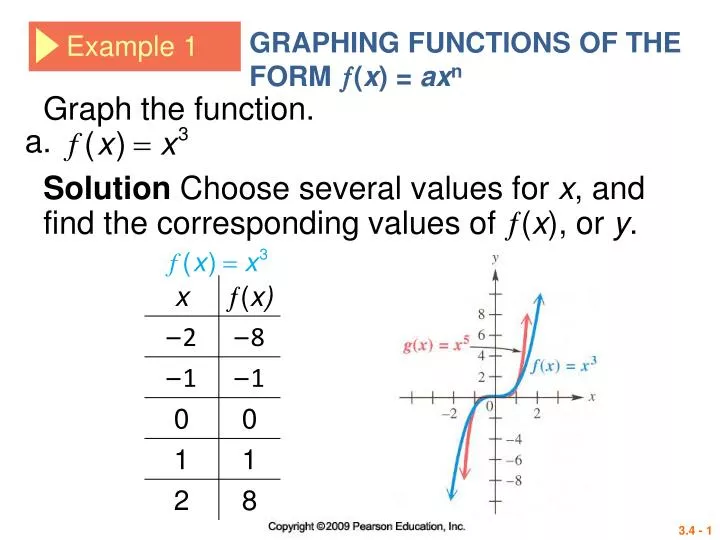
GRAPHING FUNCTIONS OF THE FORM ( x ) = ax n. Example 1. Graph the function. a. Solution Choose several values for x , and find the corresponding values of ( x ), or y.

E N D
GRAPHING FUNCTIONS OF THE FORM (x) = axn Example 1 Graph the function. a. Solution Choose several values for x, and find the corresponding values of (x), or y.
If the zero has even multiplicity, the graph is tangent to the x-axis at the corresponding x-intercept (that is, it touches but does not cross the x-axis there).
If the zero has odd multiplicity greater than one, the graph crosses the x-axisand is tangent to the x-axis at the corresponding x-intercept. This causes a change in concavity, or shape, at the x-intercept and the graph wiggles there.
Turning Points and End Behavior The previous graphs show that polynomial functions often have turning points where the function changes from increasing to decreasing or from decreasing to increasing.
Turning Points A polynomial function of degree n has at most n – 1 turning points, with at least one turning point between each pair of successive zeros.
End Behavior The end behavior of a polynomial graph is determined by the dominating term, that is, the term of greatest degree. A polynomial of the form has the same end behavior as .
End Behavior of Polynomials • Suppose that axn is the dominating term of a polynomial function of odd degree. • If a > 0, then as and as • Therefore, the end behavior of the graph is of the type that looks like the figure shown here. • We symbolize it as .
End Behavior of Polynomials Suppose that axn is the dominating term of a polynomial function of odd degree. 2. If a < 0, then as and as Therefore, the end behavior of the graph looks like the graph shown here. We symbolize it as .
End Behavior of Polynomials • Suppose that axn is the dominating term of a polynomial function of even degree. • If a > 0, then as • Therefore, the end behavior of the • graph looks like the graph shown here. • We symbolize it as .
End Behavior of Polynomials Suppose that is the dominating term of a polynomial function of even degree. 2. If a < 0, then as Therefore, the end behavior of the graph looks like the graph shown here. We symbolize it as .
DETERMINING END BEHAVIOR GIVEN THE DEFINING POLYNOMIAL Example 3 Match each function with its graph. A. B. C. D. Solution Because is of even degree with positive leading coefficient, its graph is C.
DETERMINING END BEHAVIOR GIVEN THE DEFINING POLYNOMIAL Example 3 Match each function with its graph. A. B. C. D. Solution Because g is of even degree with negative leading coefficient, its graph is A.
DETERMINING END BEHAVIOR GIVEN THE DEFINING POLYNOMIAL Example 3 Match each function with its graph. A. B. C. D. Solution Because function h has odd degree and the dominating term is positive, its graph is in B.
DETERMINING END BEHAVIOR GIVEN THE DEFINING POLYNOMIAL Example 3 Match each function with its graph. A. B. C. D. Solution Because function k has odd degree and a negative dominating term, its graph is in D.
Graphing Techniques We have discussed several characteristics of the graphs of polynomial functions that are useful for graphing the function by hand. A comprehensive graph of a polynomial function will show the following characteristics: 1. all x-intercepts (zeros) 2. the y-intercept 3. the sign of (x) within the intervals formed by the x-intercepts, and all turning points 4. enough of the domain to show the end behavior. In Example 4, we sketch the graph of a polynomial function by hand. While there are several ways to approach this, here are some guidelines.