Download
1 / 31
340 likes | 628 Vues
Loss Given Default and Credit Portfolio Risk. Jon Frye Senior Economist Federal Reserve Bank of Chicago Jon.Frye@chi.frb.org Symposium on Enterprise Wide Risk Management Chicago, April 26, 2004

E N D
Loss Given Default and Credit Portfolio Risk Jon Frye Senior Economist Federal Reserve Bank of Chicago Jon.Frye@chi.frb.org Symposium on Enterprise Wide Risk Management Chicago, April 26, 2004 The views expressed are the author’s and do not necessarily represent the views of the management of the Federal Reserve Bank of Chicago or the Federal Reserve System.
What is loss given default (LGD)? • LGD is the fraction lost when obligors default. • Generally, LGD is reduced by • Seniority • Security, such as loan collateral • Guarantees, … • Therefore, guaranteed senior secured bank loans tend to have low LGD. • Subordinated bonds tend to have high LGD.
What are the main themes today? • When the default rate is high, the loss-given-default rate (LGD) tends to be high. • LGD variation can significantly affect credit loss. • This connection is missing in most portfolio credit risk models (but it could be added). • There won't be much math (today).
Three steps of risk management • Risk identification • LGDs rise with the default rate. • This is becoming the consensus of credit risk modelers. • Today's presentation fits into this step. • Risk analysis • Quantify the strength of the correlation, and project the level of LGD in severe economic downturns. • Risk resolution • Incorporate varying LGD into portfolio risk models. • Models have been introduced to do this.
A step towards risk identification • "A False Sense of Security" Risk, August 2003 • "Low" LGDs appear especially sensitive to the default rate. • "Low" LGDs appear more sensitive to high default years than the default rate itself. • It is good to reduce LGD, but… • How "first generation" credit risk models (ones that use static LGD) work. • How systematic LGD variation would fit in.
Default universe • Moody's Corporate Default Database, 1983-01 • No WorldCom, NTL, Intermedia, Nextel… • Default universe = US non-financial issuers • Broad and narrow industries must be non-financial • Excludes "Insurance, Property and casualty" • Excludes "Industrial, Insurance" • Contains both rated bonds and rated loans • Default is late payment, bankruptcy, etc.
High and low default years Bad years
LGD universe • Defaulted USD issues with post-default price • LGD = 100 – bid price 2 to 8 weeks after default. • Take an average if a default involves more than one issue of the same debt type, e.g., • Guaranteed sen. sec. revolving credit facilities • Senior secured notes • Some analysts prefer "final" to "market" LGD. • Record the cash flows of the defaulted instrument. • Discount to default date using the appropriate rate.
Loan data cautions • A smaller proportion of loans is rated, as compared to bonds. • First Moody's loan rating assigned in 1995. • Rated loans may differ systematically from unrated. • A smaller proportion of defaulted loans have observed prices, as compared to bonds. • The prices of defaulted loans are hard to observe, let alone to random sample.
Data set detail Good years Bad years Rating-years 22,129 7,366 Defaults 381 369 Bonds with price 535 544 Loans with price 32 73 • Moody's assigns to each issue • a level of seniority (senior secured, senior unsecured, senior subordinated, or subordinated) • a debt type (among 121 debt types).
LGD data detail • There are 960 LGDs within 121 debt types. • Each LGD is the average in a debt type in a default. • 173 Senior secured LGDs are in 47 debt types • 32 defaulted guaranteed sen. sec. revolving credit facilities • 12 defaulted senior secured notes • 129 additional LGDs are in 45 debt types • 269 Senior unsecured LGDs are in 37 debt types • 161 Senior subordinated LGDs are in 16 debt types • 357 Subordinated LGDs are in 35 debt types
Comparing good and bad years • 49 debt types have defaults in both subperiods. • This includes 859 of the 960 LGDs. • Scatter plot shows average LGD in low default years and average LGD in high default years. • The size of a bubble indicates the total number of LGDs within the debt type. • Number of LGDs per debt type ranges 2 to 111.
Comparing good and bad years • Most debt types have greater LGD in high default periods, compared to "good" years. • Only two debt types had bad-year average LGD less than 30%. • This is irrespective of good-year performance.
LGD rises in bad years • Only two debt types have bad year LGD < 30%. • LGD rises (is above 45º line) in bad years. • Non-parametric test significance = 0.001% • LGD rises for nearly every debt type. • Debt types that do not suffer in bad years are few in number and each comprises few defaults. • The effect is not driven by particular industries (eg, telecom), but is pervasive.
Practical importance of LGD risk • Practical importance for two debt types. • The proportional variation in LGD compared to the proportional variation in the default rate. • The variation of default has practical importance. • Surprisingly, low LGDs vary more than default rates. • The average variation across the spectrum of good-year average LGD.
Practical importance of LGD risk • Senior discount notes (N=7) • Good year average LGD = 70.5 • Bad year average LGD = 86.6 • Difference = 16.1 • Percentage difference = 23% • Gtd. senior secured tranche B term loan (N=7) • Good year average LGD = 16.5 • Bad year average LGD = 33.3 • Difference = 16.8 • Percentage difference = 102%
The effects of bad years • "Bad years" are defined by high default rates. • Default rates must respond to the bad years. • Nonetheless, average LGD rates respond more. • The proportionate response of low LGDs exceeds the response of default rates. • If the year-to-year variation in the default rate is important enough to model, so is LGD variation!
Average effect on all debt types • In a regression involving all LGDs, LGDij = LGDj + 0.17 BAD + eij • Average bad year LGDs were 17 points greater. • The t statistic equals 10.7. • The regression summarizes the data; it does not indicate LGD in a severe economic downturn. • This can help identify the deals that have been most sensitive to high default periods.
Implications for risk management • Pricing of credit-risky assets • Stress testing • Credit risk modeling
Pricing credit-risky assets • Systematic LGD variation implies greater risk. • Greater risk implies greater required return. • Therefore, LGD variation deserves a role in the pricing of credit risky assets. • To date, most of the work on credit risk has focused solely on the default rate side.
Stress testing • Investors sometimes stress test their portfolios under adverse scenarios. • An adverse scenario should be worse than the episodes experienced to date. • All years experienced so far are "good years" from the stress test perspective. • Stress scenarios should include higher default rates and simultaneously higher LGD rates. • The amount higher should be guided by historical experience and by risk modeling.
Credit risk modeling • Calibration models can produce statistical estimates of the LGD correlation. • Depressing Recoveries assumes that LGD is normally distributed, with mean that depends on the economy. • Collateral Damage assumes the assets supporting recovery are normally distributed (with a mean that depends on the economy), but the value is observed only after default. • Production models take the correlation estimate as given and compute the risk of a portfolio.
What's next for this risk analysis • Use the granular data presented here to calibrate alternative credit risk models. • Test for differences between bonds and loans. • Estimate the appropriate correlations. • These could be used in "ground-up" risk models that allow for systematic LGD risk. • Develop a rule of thumb approximation for LGD in a severe economic downturn. • This could be used in first generation credit risk models to better assess LGD risk.
Summary for now • LGD have been greater in high default years, and much greater for some kinds of debt. • Low LGDs have risen the most, proportionally. • Granular analysis is required to estimate the underlying correlation. • Correlation increases risk in a credit model, and LGD correlation is no exception.
References • Collateral Damage • Risk Magazine, April 2000 • Depressing Recoveries • Risk Magazine, November 2000 • A False Sense of Security • Risk Magazine, August 2003 • http://www.chicagofed.org/bankinforeg /bankregulation/capitalrisk.cfm
Loss Given Default and Credit Portfolio Risk Jon Frye Senior Economist Federal Reserve Bank of Chicago Jon.Frye@chi.frb.org Symposium on Enterprise Wide Risk Management Chicago, April 26, 2004 The views expressed are the author’s and do not necessarily represent the views of the management of the Federal Reserve Bank of Chicago or the Federal Reserve System.