Download
1 / 43
490 likes | 823 Vues
Introduction to Graph Mining. Sangameshwar Patil Systems Research Lab TRDDC, TCS, Pune. Outline. Motivation Graphs as a modeling tool Graph mining Graph Theory: basic terminology Important problems in graph mining FSG: Frequent Subgraph Mining Algorithm. Motivation.

E N D
Introduction to Graph Mining Sangameshwar Patil Systems Research Lab TRDDC, TCS, Pune
Outline • Motivation • Graphs as a modeling tool • Graph mining • Graph Theory: basic terminology • Important problems in graph mining • FSG: Frequent Subgraph Mining Algorithm
Motivation • Graphs are very useful for modeling variety of entities and their inter-relationships • Internet / computer networks • Vertices: computers/routers • Edges: communication links • WWW • Vertices: webpages • Edges: hyperlinks • Chemical molecules • Vertices: atoms • Edges: chem. Bonds • Social networks (Facebook, Orkut, LinkedIn) • Vertices: persons • Edges: friendship • Citation/co-authorship network • Disease transmission • Transport network (airline/rail/shipping) • Many more…
Motivation: Graph Mining • What are the distinguishing characteristics of these graphs? • When can we say two graphs are similar? • Are there any patterns in these graphs? • How can you tell an abnormal social network from a normal one? • How do these graph evolve over time? • Can we generate synthetic, but realistic graphs? • Model evolution of Internet? • …
Terminology-I • A graph G(V,E) is made of two sets • V: set of vertices • E: set of edges • Assume undirected, labeled graphs • Lv: set of vertex labels • LE: set of edge labels • Labels need not be unique • e.g. element names in a molecule
Terminology-II • A graph is said to be connected if there is path between every pair of vertices • A graph Gs (Vs, Es) is a subgraph of another graph G(V, E) iff • Vs is subset of V and Es is subset of E • Two graphs G1(V1, E1) and G2(V2, E2) are isomorphicif they are topologically identical • There is a mapping from V1 to V2 such that each edge in E1 is mapped to a single edge in E2 and vice-versa
Terminology-III: Subgraph isomorphism problem • Given two graphs G1(V1, E1) and G2(V2, E2): find an isomorphism between G2 and a subgraph of G1 • There is a mapping from V1 to V2 such that each edge in E1 is mapped to a single edge in E2 and vice-versa • NP-complete problem • Reduction from max-clique or hamiltonian cycle problem
Need for graph isomorphism • Chemoinformatics • drug discovery (~ 1060 molecules ?) • Electronic Design Automation (EDA) • designing and producing electronic systems ranging from PCBs to integrated circuits • Image Processing • Data Centers / Large IT Systems
Other applications of graph patterns • Program control flow analysis • Detection of malware/virus • Network intrusion detection • Anomaly detection • Classifying chemical compounds • Graph compression • Mining XML structures • …
Example*: Frequent subgraphs *From K. Borgwardt and X. Yan (KDD’08)
An Efficient Algorithm for Discovering Frequent Sub-graphs IEEE ToKDE 2004 paper by Kumarochi & Karypis
Outline • Motivation / applications • Problem definition • Recap of Apriori algorithm • FSG: Frequent Subgraph Mining Algorithm • Candidate generation • Frequency counting • Canonical labeling
Outline • Motivation / applications • Problem definition • Complexity class GI • Recap of Apriori algorithm • FSG: Frequent Subgraph Mining Algorithm • Candidate generation • Frequency counting • Canonical labeling
Problem Definition Given D : a set of undirected, labeled graphs σ : support threshold ; 0 < σ<= 1 Find all connected, undirected graphs that are sub-graphs in at-least σ . | D | of input graphs
Complexity • Sub-graph isomorphism • Known to be NP-complete • Graph Isomorphism (GI) • Ambiguity about exact location of GI in conventional complexity classes • Known to be in NP • But is not known to be in P or NP-C • (factoring is another such problem) • A class in its own • Complexity class GI • GI-hard • GI-complete
Outline • Motivation / applications • Problem definition • Recap of Apriori algorithm • FSG: Frequent Subgraph Mining Algorithm • Candidate generation • Frequency counting • Canonical labeling
Apriori-algorithm: Frequent Itemsets Ck: Candidate itemset of size k Lk: frequent itemset of size k Frequent: count >= min_support • Find frequent set Lk−1. • Join Step • Ck is generated by joining Lk−1 with itself • Prune Step • Any (k−1)-itemset that is not frequent cannot be a subset of a frequent k -itemset, hence should be removed.
Apriori: Example Set of transactions : { {1,2,3,4}, {2,3,4}, {2,3}, {1,2,4}, {1,2,3,4}, {2,4} } min_support: 3 L3 L1 C2 L2 {1,2,3} and {1,3,4} were pruned as {1,3} is not frequent. {1,2,3,4} not generated since {1,2,3} is not frequent. Hence algo terminates.
Outline • Motivation / applications • Problem definition • Recap of Apriori algorithm • FSG: Frequent Subgraph Mining Algorithm • Candidate generation • Frequency counting • Canonical labeling
FSG: Frequent Subgraph Discovery Algo. • ToKDE 2004 • Updated version of ICDM 2001 paper by same authors • Follows level-by-level structure of Apriori • Key elements for FSG’s computational scalability • Improved candidate generation scheme • Use of TID-list approach for frequency counting • Efficient canonical labeling algorithm
FSG: Basic Flow of the Algo. • Enumerate all single and double-edge subgraphs • Repeat • Generate all candidate subgraphs of size (k+1) from size-k subgraphs • Count frequency of each candidate • Prune subgraphs which don’t satisfy support constraint Until (no frequent subgraphs at (k+1) )
Outline • Motivation / applications • Problem definition • Recap of Apriori algorithm • FSG: Frequent Subgraph Mining Algorithm • Candidate generation • Frequency counting • Canonical labeling
FSG: Candidate Generation - I • Join two frequent size-k subgraphs to get (k+1) candidate • Common connected subgraph of (k-1) necessary • Problem • K different size (k-1) subgraphs for a given size-k graph • If we consider all possible subgraphs, we will end up • Generating same candidates multiple times • Generating candidates that are not downward closed • Significant slowdown • Apriori algo. doesn’t suffer this problem due to lexicographic ordering of itemset
FSG: Candidate Generation - II • Joining two size-k subgraphs may produce multiple distinct size-k • CASE 1: Difference can be a vertex with same label
FSG: Candidate Generation - III • CASE 2: Primary subgraph itself may have multiple automorphisms • CASE 3: In addition to joining two different k-graphs, FSG also needs to perform self-join
FSG: Candidate Generation Scheme • For each frequent size-k subgraph Fi , define primary subgraphs: P(Fi) = {Hi,1 , Hi,2} • Hi,1 , Hi,2 : two (k-1) subgraphs of Fi with smallest and second smallest canonical label • FSG will join two frequent subgraphs Fi and Fj iff P(Fi) ∩ P(Fj) ≠ Φ This approach correctly generates all valid candidates and leads to significant performance improvement over the ICDM 2001 paper
Outline • Motivation / applications • Problem definition • Recap of Apriori algorithm • FSG: Frequent Subgraph Mining Algorithm • Candidate generation • Frequency counting • Canonical labeling
FSG: Frequency Counting • Naïve way • Subgraph isomorphism check for each candidate against each graph transaction in database • Computationally expensive and prohibitive for large datasets • FSG uses transaction identifier (TID) lists • For each frequent subgraph, keep a list of TID that support it • To compute frequency of Gk+1 • Intersection of TID list of its subgraphs • If size of intersection < min_support, • prune Gk+1 • Else • Subgraph isomorphism check only for graphs in the intersection • Advantages • FSG is able to prune candidates without subgraph isomorphism • For large datasets, only those graphs which may potentially contain the candidate are checked
Outline • Motivation / applications • Problem definition • Recap of Apriori algorithm • FSG: Frequent Subgraph Mining Algorithm • Candidate generation • Frequency counting • Canonical labeling
Canonical label of graph • Lexicographically largest (or smallest) string obtained by concatenating upper triangular entries of adj. matrix (after symmetric permutation) • Uniquely identifies a graph and its isomorphs • Two isomorphic graphs will get same canonical label
Use of canonical label • FSG uses canonical labeling to • Eliminate duplicate candidates • Check if a particular pattern satisfies the downward closure property • Existing schemes don’t consider edge-labels • Hence unusable for FSG as-is • Naïve approach for finding out canonical label is O( |v| !) • Impractical even for moderate size graphs
FSG: canonical labeling • Vertex invariants • Inherent properties of vertices that don’t change across isomorphic mappings • E.g. degree or label of a vertex • Use vertex invariants to partition vertices of a graph into equivalent classes • If vertex invariants cause m partitions of V containing p1, p2, …, pm vertices respectively, then number of different permutations for canonical labeling π (pi !) ; i = 1, 2, …, m which can be significantly smaller than |V| ! permutations
FSG canonical label: vertex invariant - I • Partition based on vertex degrees and labels Example: number of permutations reqd = 1 ! x 2! x 1! = 2 Instead of 4! = 24
FSG canonical label: vertex invariant - II • Partition based on neighbour lists • Describe each adjacent vertex by a tuple < le, dv, lv > le = edge label dv = degree lv = label
FSG canonical label: vertex invariant - II • Two vertices in same partition iff their nbr. lists are same • Example: only 2! Permutations instead of 4! x 2!
FSG canonical label: vertex invariant - III • Iterative partitioning • Different way of building nbr. list • Use pair <pv, le> to denote adjacent vertex • pv = partition number of adj. vertex c • le = edge label
FSG canonical label: vertex invariant - III Iter 1: degree based partitioning
FSG canonical label: vertex invariant - III Nbr. List of v1 is different from v0, v2. Hence new partition introduced. Renumber partitions and update nbr. lists. Now v5 is different.
Next steps • What are possible applications that you can think of? • Chemistry • Biology • We have only looked at “frequent subgraphs” • What are other measures for similarity between two graphs? • What graph properties do you think would be useful? • Can we do better if we impose restrictions on subgraph? • Frequent sub-trees • Frequent sequences • Frequent approximate sequences • Properties of massive graphs (e.g. Internet) • Power law (zipf distribution) • How do they evolve? • Small-world phenomenon (6 hops of separation, kevin beacon number)