Download
1 / 23
240 likes | 400 Vues
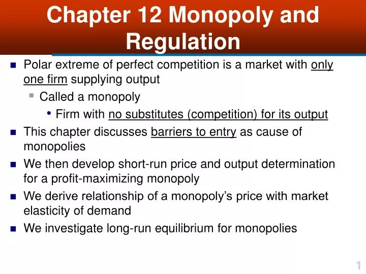
Chapter 12 Monopoly and Regulation. Polar extreme of perfect competition is a market with only one firm supplying output Called a monopoly Firm with no substitutes (competition) for its output This chapter discusses barriers to entry as cause of monopolies

E N D
Chapter 12 Monopoly and Regulation • Polar extreme of perfect competition is a market with only one firm supplying output • Called a monopoly • Firm with no substitutes (competition) for its output • This chapter discusses barriers to entry as cause of monopolies • We then develop short-run price and output determination for a profit-maximizing monopoly • We derive relationship of a monopoly’s price with market elasticity of demand • We investigate long-run equilibrium for monopolies
Barriers to Entry • Cause of a monopoly is barriers (obstacles) to entry • Barriers to entry are anything that allow existing firms to earn pure profits • One type of a legal monopoly is established by a state or federal government awarding only one firm an exclusive franchise to provide a commodity • Government may do so because there are increasing returns to scale over a wide range of output • If society deems that unrestricted competition among firms in an industry is undesirable • Government may establish a legal monopoly by granting a firm exclusive rights to operate • For example, patents • Technological barriers to entry may result when a firm’s technology results in decreasing LAC over a wide range of output, knowledge of a low-cost productive technique, or control of a strategic resource • Termed natural monopolies • Because market forces establish monopoly
Price and Output Determination • Objective of monopolies • Maximize profits • First determine profit-maximizing output • Then determine price required to sell output • Alternatively, they can first determine profit-maximizing price • Then from market demand curve determine level of output that can be sold at this price • Resulting profit-maximizing price/output combination will be the same • Regardless of which method is employed • Market demand curve is downward sloping • If a monopoly reduces output, price it receives for this output will increase
Price and Output Determination • Monopoly has control over market price • A price maker • Consider following linear market demand curve • AR = p = a – bQ • TR = (AR)Q = pQ = aQ – bQ2 • MR = ∂TR/∂Q = a – 2bQ = a – bQ – bQ = AR - bQ • Where a, b > 0 • For a linear demand curve, MR is twice as steep as AR • Illustrated in Figure 12.1
Price and Output Determination • In Figure 12.1, AR is falling as firm increases output • Because consumers are willing and able to purchase more of commodity at lower level of AR (price) • Falling AR implies that MR is below it • MR is equal to AR plus adjustment factor, -bQ • Given -b <0 (falling AR), then MR <AR • For a given level of output, MR <AR • For a firm to sell an additional unit of output it must lower its price on all units to be sold, not just on additional units • Adjustment factor, -bQ, accounts for this condition • For each additional output sold, price falls by -b • Multiplying this fall in price by number of units sold • Results in adjustment to AR for determining MR
Profit Maximization • Mathematically, short-run profit is maximized by • F.O.C. is • ∂/∂Q = ∂TR/∂Q = ∂STC/ ∂Q = 0 = MR(Q) – SMC(Q) = 0 • Profit-maximizing monopoly will equate MR to SMC to determine its optimal level of output • Profit-maximizing output Q* corresponds to where MR =SMC • Illustrated in Figure 12.2 • Firm will produce Q* units of output and, given market demand curve QD, it can sell all of this output at p* • p* corresponds to level of output Q* that consumers are willing and able to purchase
Profit Maximization • SMC curve for a monopoly determines profit-maximizing price and output • However, in contrast to perfect competition, SMC curve above SAVC is not monopoly’s short-run supply curve • In Figure 12.2, if SMC curve for a monopoly is a supply curve, at a price of p* • Firm would be willing and able to supply Q'units of output • Although firm is able to supply Q'at p*, it is unwilling to supply it • Profit-maximizing output is Q* • Firm can sell all output at p* • Cannot determine a monopoly’s short-run supply curve without restrictive assumptions • Note that same factors that shift a monopoly’s short-run supply curve also shift SMC curve in same direction
Profit Maximization • In Figure 12.2, price p* is above SATC* for output level Q* • Indicates monopoly is earning a pure profit • Represented by shaded area SATC*p*AB • TR is represented by area 0p*AQ* • STC is represented by area 0(SATC*)BQ* • Difference is pure profit • As illustrated in Figure 12.3, in short run a monopoly can also earn only a normal profit • When p* = SATC* • Due to increased input prices or a decrease in demand for its output • In this case, TR* =STC*, area 0p*AQ*
Figure 12.3 Short-run profit maximization for a monopoly earning a normal profit
Profit Maximization • In short run, a monopoly can also operate at a loss if demand falls or costs increase • Illustrated in Figure 12.4 • Losses represented by shaded area p*(SATC*)BA • As long as price is above SAVC a monopoly will continue to operate in short run • Monopoly will cover all of its STVC and have some revenue left over for paying a portion of its TFC • Monopoly minimizes its losses by operating • If price falls below SAVC, monopoly is unable to cover its STVC • Will minimize losses by shutting down • In summary, a monopoly can earn a pure profit, a normal profit, or can operate at a loss in short run • Firm’s level of profit is not an indicator of its degree of monopoly power • Percentage markup in price over marginal cost, (p -SMC )/p, is indicator of monopoly power
Figure 12.4 Price and output determination for a monopoly operating at a loss
Lerner Index • Regardless of its level of monopoly power • Firm only operates in elastic portion of demand curve • Given SMC > 0, a profit-maximizing firm will equate MR = SMC >0 • Using product rule of differentiation and recalling TR =pQ • Relationships of MR to price and to elasticity of market demand are • MR = dTR/dQ = p + (∂p/∂Q)Q • MR is equal to price plus adjustment factor
Lerner Index • For each additional output sold price falls by ∂p/∂Q • Multiplying this by number of units sold results in adjustment to AR for determining MR • Factoring out price from right-hand side of MR =p + (∂p/∂Q)(Q) yields relationship between MR and elasticity of demand • MR =p[1 + (∂p/∂Q)(Q/p)] = p(1 + 1/D) • Where /D =(∂Q/∂p)(p/Q)], own-price elasticity of demand • For MR >0, (1 +1/D)> 0 • Which implies D < -1 (elastic) • If D > 1 (inelastic) • MR =dTR/dQ <0 • Decrease in Q will increase TR • Given dSTC/dQ >0, STC decreases with this decrease in Q • Yielding an increase in pure profit • Profit-maximizing firm can continue to reduce Q and increase profit within inelastic portion of demand curve • Firm will reduce output until it is in elastic portion of demand curve • Where MR =SMC • Table 12.1 summarizes relationships between demand elasticity and marginal revenue
Lerner Index • At MR = SMC • MR = p(1 + 1/D) = SMC • Solving for p gives • p = SMC/(1 + 1/D) • Under perfect competition, a firm is facing a perfectly elastic demand curve • So 1/D =0, indicating condition of p =SMC for profit maximization • Instead, a monopoly charges a higher price • Since it only operates on elastic portion of demand curve • Then 0 <(1 +1/D) <1, so p >SMC • A measure of degree of monopoly power is percentage markup in price over marginal cost (p -SMC )/p • Specifically, given p(1 + 1/D) = SMC and solving for (p -SMC )/p yields Lerner Index (LI) • LI = (p – SMC)/p = -1/D • Lerner Index varies between 0 and 1 and measures percentage markup in price due to monopoly power • Relative difference in price and marginal cost is dependent on elasticity of demand
Lerner Index • Under perfect competition, p =SMC, D = -, so LI= 0 • Firm is exercising zero monopoly power • If D = -1, then LI =1, indicating existence of monopoly power • At -1 ≥ D > -, corresponding to 0 <LI ≤1, a relative wedge between price and SMC exists • Magnitude of this wedge is determined by elasticity of demand • When demand curve becomes less elastic, wedge increases and LI approaches 1 • Wedge for a profit-maximizing firm without close substitutes will be large relative to a firm in a market with many competitors • Monopoly is concerned with effect high price has on consumption • When consumers react to a price increase by greatly reducing their demand • Monopoly will not charge highest price it can for its output • It will determine elasticity of demand for its output and calculate LI • Table 12.2 lists measurements of Lerner Index for steel and semiconductor industries
Table 12.2 Measurements of the Lerner Index for the Steel and Semiconductor Industries
Long-Run Equilibrium • Long-run equilibrium for a monopoly is illustrated in Figure 12.5 • SATC and LAC curves are tangent at firm’s profit-maximizing output level Q* • Where SMC =LMC =MR • At this equilibrium output and price (Q*, p*), firm is earning a normal profit • In long run, firm can earn only a normal profit • If it had been earning a pure profit in short run, when firm is sold in the long run • New owners will pay a higher price for firm than if it had been earning only a normal profit • Increases cost of operation • Results in upward shift of cost curves
Long-Run Equilibrium • Competition for purchasing firm will result in cost curves for new owners shifting up to point of zero pure profit (normal profit) • Market price for firm will increase until, in long run, all short-run pure profits are squeezed out • p =SATC =LAC • Even if firm is not sold, cost of production (in terms of implicit cost) will increase over time • In long run, a firm that earned a short-run pure profit will be worth more, say $100,000 • Thus, owners of firm have a higher implicit cost of production • Their opportunity cost for operating firm has increased because they could sell firm and receive this increase in price ($100,000) and invest it in another activity • Called opportunity cost of capital • If alternative activity had an annual rate of return of 10%, then firm’s implicit cost of production would be $10,000 higher • Short-run pure profit is converted into implicit cost • Alternatively, if firm had been operating at a loss in short run, firm will not be worth as much • Cost curves will shift downward, resulting in a long-run normal profit
Long-Run Equilibrium • The worth of a monopoly based on its long-run pure-profit potential is called monopoly rents • Rent a possible entrant would be willing to pay for monopoly • Given positive monopoly rents, associated opportunity cost exists that result in only long-run normal profits • Without considering that cost adjusts to rents, it is possible to assume a monopoly will earn a long-run pure profit • This fact is particularly important in basic business decision-making • Since firms, even those with monopoly power, can only make a pure profit in short run • Owners of firms cannot continue their present activities and expect continued pure profits • If they want to continue to reap pure profit, must anticipate market trends • So as to sell their firms when conditions are right and be early entrants into markets where firms are earning short-run pure profits • However, many individuals or firms either lack this knowledge or are unwilling to act • Because they can maximize their utility by staying in a particular activity even if it means earning only a normal profit