Download
1 / 11
120 likes | 287 Vues
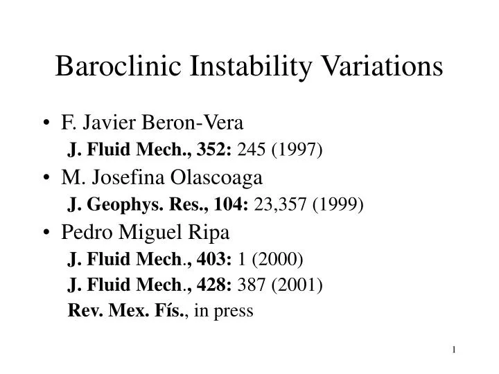
Baroclinic Instability Variations. F. Javier Beron-Vera J. Fluid Mech., 352: 245 (1997) M. Josefina Olascoaga J. Geophys. Res., 104: 23,357 (1999) Pedro Miguel Ripa J. Fluid Mech . , 403: 1 (2000) J. Fluid Mech . , 428: 387 (2001) Rev. Mex. Fís. , in press. Outline. Background

E N D
Baroclinic Instability Variations • F. Javier Beron-Vera J. Fluid Mech., 352: 245(1997) • M. Josefina Olascoaga J. Geophys. Res., 104: 23,357(1999) • Pedro Miguel Ripa J. Fluid Mech., 403: 1(2000) J. Fluid Mech., 428: 387(2001) Rev. Mex. Fís., in press
Outline • Background • Generalizing Two-field models • Charney Numbers – Arnold-1 • Low- and Short-wave cutoff – Arnold-2 • Components “resonance” • Rossby Waves resonance • Bounds on the growth of perturbations
Eady (1949): β = 0, rigid horizontal boundaries Blumsack & Gierasch (1972): β = 0, sloping bottom Fukamachi et al. (1995):β = 0, free bottom, βT = 0 (topographic) Beron-Vera (1997):β = 0, free bottom, βT 0 Lindzen (1994): β 0, but q uniform. Phillips (1951): β 0, rigid horizontal boundaries Bretherton (1966): β = 0, rigid sloping boundaries Olascoaga (1999) : β 0, free bottom , βT 0
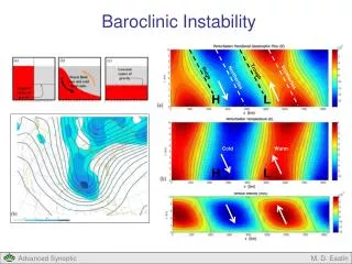
Basic Flow: Two Charney # (beta/shear) Outside the wedge, a hamiltonian (“energy”) is H > 0: nonlinear stability (Arnold’s First Theorem)
Enter another variable: the perturbation wavenumber κ All hamiltonians are sign independent for κL(b,bT) < κ < κS(b,bT) Notice the finite region for κL(b,bT) = 0
Growth Rate along different directions in the (b,bT) plane (see color coded regions in slide 5) • If the advection of a q field by the other q field is arbitrarely neglected, these uncoupled components “resonate” along the blue curve. This “explains” the instability onset. (If shear 0 then b, bT along b/bT = const.) • Maximum growth rate near b + bT 0
Resonance of Rossby Waves The conditionb + bT 0 corresponds to the cancellation of both beta effects+ T 0: near resonance of true waves.This “explains” the maximum growth rate.
Bounding the wavy part of the perturbation qj,à la Shepherd, or the whole perturbation qj
Conclusions • Generalized Phillips-like or Eady-like model: • either two layers with constant density and variable potential vorticity orone layer with constant potential vorticity and variable boundary densities • free boundary and/or fixed topography • Necessary and sufficient stability conditions • “Resonance” of uncouple dynamical fields • At the cancellation of planetary and topographic beta effects: • resonance of Rossby waves • maximum growth rate • perturbation growth bounds are trivial