Download
1 / 103
1.16k likes | 1.25k Vues
Chapter 11 Unicast Routing Protocols (RIP, OSPF, and BGP). 11.1 Introduction. An internet is a combination of networks connected by routers A metric is a cost assigned for passing through a network.

E N D
11.1 Introduction • An internet is a combination of networks connected by routers • A metric is a cost assigned for passing through a network. • the total metric of a particular route is equal to the sum of the metrics of networks that comprise the route. • the router chooses the route with the shortest (smallest) metric • RIP (Routing Information Protocol) : treating each network equals. • The cost of passing through each network is the same. • so if a packet passes through 10 networks to reach the destination, the total cost is hop counts.
Introduction • OSPF(Open Shortest Path First) • allowing the administrator to assign a cost for passing through a network based on the type of service required. • A route through a network can have different costs (metrics) • BGP (Border Router Protocol) • Criterion is the policy, which can be set by the administrator. • Policy defines what paths should be chosen. • Static and Dynamic tables • Unicast Routing and Multicast Routing
11.2 Intra and Inter-Domain Routing • Because an internet can be so large, one routing protocol cannot handle the task of updating routing tables of all routers. • So, an internet is divided into autonomous systems. • An autonomous system (AS) is a group of networks and routers under the authority of a single administration. • Intradomain routing • used for the routing inside an autonomous system • Interdomain routing • used for the routing between autonomous systems
Intra and Inter-Domain Routing (Cont’d) • Popular routing protocols
11.3 Distance Vector Routing • In distance vector routing, the least cost route between any two nodes is the route with minimum distance. In this protocol each node maintains a vector (table) of minimum distances to every node • The table at the each node also guides the packet to the desired node by showing the next stop in the route (next-hop routing) • Distance Vector Routing • each router periodically shares its knowledge about the entire internet with neighbors • the operational principles of this algorithm • Sharing knowledge about the entire autonomous system • Sharing only with neighbors • Sharing at regular intervals (ex, every 30 seconds) and when there is a change
Bellman-Ford Algorithm The shortest distance and the cost between a node and itself is initialized to 0 The shortest distance between a node and any other node is set to infinity. The cost between a node and any other node should be given. The algorithm repeat until there is no more change in the shortest distance vector
A graph for the Bellman-Ford Algorithm If we know the cost between each pair of nodes, we can use the algorithm to find the least cost.
Distance Vector Routing Algorithm • In distance vector routing, each node shares its routing table with its immediate neighbors periodically and when there is a change.
Distance Vector Routing Algorithm In distance vector routing, the cost is normally hop counts. So the cost between any two neighbors is set to 1. Each router needs to updates its routing table asynchronously, where it has received some information from its neighbors. In other words, each router executes part of the whole algorithm in the Bellman-Ford algorithm. Processing is distributive After a router has updated its routing table, it should send the result to its neighbor so that they can also update their routing table Each router should keep at least three pieces of information for each route: destination network, the cost, and the next hop. We refer to the whole routing table as Table, to the row i in the table as Tablei. dest, Tablei.cost, and Tablei.next. We refer to information about each route received from a neighbor as R, which has only two piece of information : R.dest and R.cost. The next hop is not included in the received record because it is the source address of the sender
Example 11.1 Figure 11.5 shows the initial routing table for an AS. Note that the figure does not mean that all routing tables have been created at the same time; each router creates its own routing table when it is booted
Example 11.2 Now assume router A sends four records to its neighbors, routers B, D, and C. Figure 11.6 shows the changes in B’s routing table when it receive these records. We leave the changes in the routing tables of other neighbor as exercise.
Count to Infinity • A problem of distance vector routing • Any decrease in cost (bad news) propagates quickly • Any increase in cost (good news) propagates slowly • If a link broken, every other router should be aware of it immediately • The problem is referred to as count to infinity • Ex) Two-node loop
Some Remedies for Instability • Defining Infinity • Redefine infinity to a smaller number, such as 16. • Split horizon • Instead of flooding the table through each interface, each node sends only part of its table through each interface • Split horizon and poison reverse • The split horizon strategy can be combined with the poison reverse strategy. Node can replace the distance with infinity as warning.
11.4 RIP • The Routing Information Protocol (RIP) is an intradomain routing protocol used inside an autonomous system. It is a very simple protocol based on distance vector routing. • The destination in a routing table is a network, which means the first column defines a network address. • A metric in RIP is called a hop count; distance; defined as the number of links (networks) that have to be used to reach the destination.
RIP (cont’d) • RIP Message Format • Command : request (1) or response (2) • Version • Family : For TCP/IP the value is 2 • Address : destination network address • Distance : defining the hop count from the advertising router to the destination network * Part of the message (entry) is repeated for each destination network.
Request • Sent by a router that has just come up or by a router that has some time-out entries.
Response • Response • solicited response • is sent only in answer to a request • containing information about the destination specified in the corresponding request • unsolicited response • is sent periodically, every 30 seconds • containing information covering the whole routing table
Example 11.4 Figure 11.13 shows the update message sent from router R1 to router R2 in Figure 11.10. The message is sent out of interface 130.10.0.2. The message is prepared with the combination of split horizon and poison reverse strategy in mind. Router R1 has obtained information about networks 195.2.4.0, 195.2.5.0, and 195.2.6.0 from router R2. When R1 sends an update message to R2, it replaces the actual value if the hop counts for these three networks with 16 (infinity) to prevent any confusion for R2. The figure also shows the table extracted from the message. Router R2 uses the source address of the IP datagram carrying the RIP message from R1 (130.10.02) as the next hop address. Router R2 also increments each hop count by 1 because the values in the message are relative to R1, not R2
Timers in RIP • Periodic timer : controlling the advertisements of regular update messages • Expiration timer : governing the validity of a route • The garbage collection timer : advertising the failure of a route
Timers in RIP • Periodic timer • controlling the advertising of regular update messages • using random number between 25 to 35 seconds • Expiration timer • In normal situation, the new update for a route occurs every 30 seconds • But, if there is a problem on an Internet and no update is received within the allotted 180 seconds, the route is considered expired and the hop count of the route is set to 16. • Each router has its own expiration timer. • Garbage Collection Timer • When the information about a route becomes invalid, the router continues to advertise the route with a metric value of 16 and the garbage collection timer is set to 120 sec for that route • When the count reaches zero, the route is purged from the table.
Example 11.5 A routing table has 20 entries. It does not receive information about five routes for 200 seconds. How many timers are running at this time? The timers are listed below: Periodic timer: 1 Expiration timer: 20 - 5 = 15 Garbage collection timer: 5
RIP Version 2 • Designed for overcoming some of the shortcomings of version 1 • Replaced fields in version 1 that were filled with 0s for the TCP/IP protocols with some new fields • Can use classless addressing
Message Format • RIP version 2 format • Route Tag :carrying information such as the autonomous system number • Subnet mask : carrying the subnet mask • Next-hop address : showing the next hop • In case that shares a network backbone by two ASs, the message can define the router to which the packet should go next
Classless Addressing • The most important difference between two version of RIP • RIPv2 adds one field for the subnet mask, which can be used to define a network prefix length • A group of networks can be combined into one prefix and advertised collectively
Authentication • Added to protect the message against unauthorized advertisement • Value of FFFF16 is entered in the family field • Authentication type : protocol used for authentication
Multicasting and Encapsulation • Multicasting • Using the multicast address 224.0.0.9 to multicast RIP messages only to RIPv2 routers in the network • Encapsulation of RIP messages • encapsulated in UDP user datagram • not included a field that indicates the length of the message • Well-known port assigned to RIP in UDP is port 520
11.5 Link State Routing • In link state routing, if each node in the domain has the entire topology of the domain, the node can use Dijkstra’s algorithm to build a routing table.
Building Routing Tables • Creation of the states of the links by each node, called the link state packet or LSP. • Dissemination of LSPs to every other router, called flooding, in an efficient and reliable way • Formation of a shortest path tree for each node • Calculation of a routing table based on the shortest path tree
Formation of Shortest Path Tree • Dijkstra Algorithm
Creation and Flooding of Link State Packet (LSP) • Where there is a change in the topology of the domain • Dissemination on a periodic basis • much longer compared to distance vector routing • 60 minutes or 2 hours • The creating node sends a copy of the LSP out of each interfaces • A node that receives an LSP compares it with the copy it may already have • keeps the new one
Dijkstra’s Algorithm Continued
Example 11.6 To show that shortest path tree for each node is different, we found the shortest path tree as seen by node C