Download
1 / 30
300 likes | 435 Vues
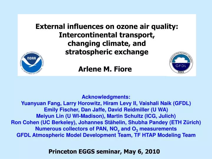
External influences on ozone air quality: Intercontinental transport, changing climate, and stratospheric exchange. Arlene M. Fiore. Acknowledgments: Yuanyuan Fang, Larry Horowitz, Hiram Levy II, Vaishali Naik (GFDL) Emily Fischer, Dan Jaffe, David Reidmiller (U WA)

E N D
External influences on ozone air quality: Intercontinental transport, changing climate, and stratospheric exchange Arlene M. Fiore Acknowledgments: Yuanyuan Fang, Larry Horowitz, Hiram Levy II, VaishaliNaik (GFDL) Emily Fischer, Dan Jaffe, David Reidmiller (U WA) Meiyun Lin (U WI-Madison), Martin Schultz (ICG, Julich) Ron Cohen (UC Berkeley), Johannes Stähelin, ShubhaPandey (ETH Zϋrich) Numerous collectors of PAN, NOy and O3 measurements GFDL Atmospheric Model Development Team, TF HTAP Modeling Team Princeton EGGS seminar, May 6, 2010
The U.S. ozone smog problem is spatially widespread, affecting ~120 million people [U.S. EPA, 2010] Counties with monitors violating newly proposed primary O3 standard in range of 0.060-.070 ppm (2006-2008 data) 4th highest daily max 8-hr O3 in 2008 Exceeds Standard (325 counties) http://www.epa.gov/air/airtrends/2010/ http://www.epa.gov/air/ozonepollution/pdfs/20100104maps.pdf
Newly proposed standards exceeded in spring in west (and SE) U.S. at “background” sites Number of days with daily max 8-hr O3 > 60 ppb SPRING SUMMER violation 2007-2009 averages using hourly O3 from CASTNetdatabase (www.epa.gov/castnet/data.html) A.M. Fiore, May 6, 2010
Brief overview of tropospheric ozone and external influences on air quality STRATOSPHERE 2. WARMING CLIMATE 3. T PAN(CH3C(O)OONO2) lightning O3 1. INTERCONTINENTAL TRANSPORT T H2O “Background” ozone NMVOCs CO CH4 + + OH NOx atmospheric cleanser Natural sources X X Fires Human activity Land biosphere Ocean Continent Continent A.M. Fiore, May 6, 2010
Evidence of intercontinental transport at northern midlatitudes: 2001 Asian dust event Clear Day April 16, 2001 Dust leaving Asian coast, April 2001 Reduced Visibility from Asian Dust over Glen Canyon, Arizona, USA Image c/o NASA SeaWiFS Project and ORBIMAGE • Intercontinental ozone transport is difficult (impossible?) to observe directly at surface [e.g., Derwent et al., 2003; Fiore et al., 2003; Goldstein et al., 2004; Jonson et al., 2005] • Estimates rely on models 3D Model Structure
Wide range in prior estimates of intercontinentalsurface ozone source-receptor (S-R) relationships NORTH AMERICA EUROPE ASIA NORTH AMERICA annual mean events events seasonal mean Surface O3 contribution from foreign region (ppbv) seasonal mean annual mean Studies in TF HTAP [2007] + Holloway et al., 2008; Duncan et al., 2008; Lin et al., 2008 Assessment hindered by different (1) methods, (2) reported metrics, (3) meteorological years, (4) regional definitions Few studies examined all seasons A.M. Fiore, May 6, 2010
Task Force on Hemispheric Transport of Air Pollution (TF HTAP): Multi-model studies to quantify & assess uncertainties in N. mid-latitude source-receptor relationships to inform CLRTAP EMEP CASTNet EANET TF HTAP REGIONS BASE SIMULATION (21 models): horizontal resolution of 5°x5° or finer 2001 meteorology each group’s best estimate for 2001 emissions methane set to 1760 ppb SENSITIVITY SIMULATIONS (13-18 models): -20% regional anthrop. NOx, CO, NMVOC emissions, individually + all together (=16 simulations) -20% global methane (to 1408 ppb) TF HTAP, 2007, 2010; Sanderson et al., GRL, 2008; Shindell et al., ACP, 2008; Fiore et al., JGR, 2009, Reidmiller et al. ACP, 2009; Casper Anenberg et al., ES&T, 2009; Jonson et al., ACPD,2010
Large inter-model range; multi-model mean generally captures observed monthly mean surface O3 Many models biased low at altitude, high over EUS+Japan in summer Good springtime/late fall simulation Mediterranean Central Europe > 1km Central Europe < 1km NE USA SW USA SE USA Surface Ozone (ppb) Japan Mountainous W USA Great Lakes USA
Model ensemble annual mean decrease in surface O3from 20% reductions of regional anthrop. O3 precursors ∑ 3 foreign = 0.45 domestic Foreign vs. “domestic” influence over NA: (1.64) Full range of 15 individual models NA “sum 3 foreign” ppbv EU “domestic” Source region: NA EU EA SA EU+EA+SA EA Spatial variability over continental- scale receptor region (NA) (see also Reidmiller et al, 2009; Lin et al., 2010) SA “import sensitivity” ppbv Fiore et al., JGR, 2009
Seasonality of surface ozone response over North American and Europe to -20% foreign anthrop. emissions Source region: SUM3 NA EAEUSA Receptor = NA Receptor = EU 15- MODEL MEAN SURFACE O3 DECREASE (PPBV) Spring max due to longer O3 lifetime, efficient transport [e.g., Wang et al., 1998; Wild and Akimoto, 2001; Stohl et al., 2002; TF HTAP 2007] Response typically smallest to SA emissions (robust across models) Similar response to EU& EA emissions over NA Apr-Nov (varies by model) NA>EA>SA over EU (robust across models) Fiore et al., JGR, 2009
SA fairly constant ~0.5 1.1 (EA), 0.7 (EU) during month with max response to foreign emissions 0.2-0.3 during month of max response to domestic emissions Monthly mean import sensitivities (surface O3 response to foreign vs. domestic emissions) Fiore et al., JGR, 2009
Models differ in estimates of surface O3 response to foreign emission changes… which are best? O3 decrease from -20% foreign emissions Over EU Over NA Fiore et al., JGR, 2009 No obvious relationship btw “base-case bias” and magnitude of source-receptor relationship (e.g., NA->EU)
PAN CH3C(O)OONO2 O3 NOx NOx+VOC PAN, O3 NOy N2O5 Models likely differ in export of O3 + precursors, downwind chemistry (PAN [Emmerson and Evans, ACP, 2009]), and transport to receptor region O3 other organic nitrates HNO3 Human activity Fires Land biosphere Ocean Ocean Continent Continent NOy partitioning (e.g., PAN vs. HNO3) influences O3 formation potential far from source region Observational evidence for O3 production following PAN decomposition in subsiding Asian plumes [e.g., Heald et al., JGR, 2003; Hudman et al., JGR, 2004; Zhang et al., 2008; Fischer et al., 2010] A.M. Fiore, May 6, 2010
Compare models with PAN measurements at high elevation sites in Europe (3 sites) and WUS (2 sites) Jungfraujoch (3.58km) c/o Emily Fischer, U Washington Mount Bachelor (2.76 km) 1. No observations from 2001; difficult to constrain models 2. How different are VOC inventories in the models? 3. What do the models say about the relative roles of regional anthrop. VOC emissions at measurement sites? Zugspitze (2.67 km) Model differences in lightning NOx affect PAN + impact of anthro. emis. [Fang et al., in review] in addition to anthrop. sources, chemistry, and transport A.M. Fiore, May 6, 2010
Strong sensitivity of exported EU O3 to large spread in EU NMVOC inventories (anthrop. NOx fairly similar across models) Annual mean surface O3 decrease over NA (ppb) from 20% decreases in anthrop. EU NMVOC Fiore et al., JGR, 2009 EU Anthrop. NMVOC Emissions (Tg C) Do the relative contributions from different source regions in the model correlate with NMVOC emissions?
Relative influence of regional O3 precursors on PAN at Mount Bachelor (OR), as estimated by the HTAP models 4 example HTAP models sampled at Mount Bachelor 0.8 0.6 0.4 0.2 0.0 Fraction of total PAN from source region EUNAEASA MOZART More EA influence Mount Bachelor, April: r2=0.85 EA/EU PAN influence correlates with EA/EU AVOC emissions Model EA_PAN/EU_PAN Individual HTAP models More EU influence Model EA_AVOC/EU AVOC A.M. Fiore, May 6, 2010
Model differences in relative contributions of source regions to PAN at Jungfraujoch, Switzerland 4 example HTAP models sampled at Jungfraujoch 0.8 0.6 0.4 0.2 0.0 MOZART Fraction of total PAN from source region EUNAEASA More EU influence Jungfraujoch, APRIL: r2=0.40 Wide range of EU NMVOC inventory contributes to model discrepancies More NA influence A.M. Fiore, May 6, 2010
Major uncertainties from sub-grid processes: Deep convection at the leading edge of the convergence band and associated pollutant export missing in global model [Lin et al., ACP, in press] Altitude (km) ppbv Altitude (km) 2001-03-07(UTC) 06UTC 04UTC 08UTC 02UTC TRACE-P c/o Meiyun Lin, UW-Madison How well do models represent mixing of free trop. air to the surface?
Summary of external influence on air quality #1: Hemispheric Transport of O3 • Benchmark for future: Robust estimates + key areas of uncertainty • “Import Sensitivities” (D O3 from anthrop. emis. in the 3 foreign vs. domestic regions): 0.5-1.1 during month of max response to foreign emis; 0.2-0.3 during month of max response to domestic emissions • Variability of O3 response to emission changes within large HTAP regions • Potential for PAN, NOy, other species, to help constrain model O3 response to emission changes • Role of “missing” processes (e.g., mesoscale)
External influence on air quality #2: Changing climate Observations c/o JeniseSwall and Steve Howard, U.S. EPA Strong relationship between weather and pollution implies that changes in climate will influence air quality A.M. Fiore, May 6, 2010
Pollution build-up during 2003 European heatwave GRG HEATWAVE Ozone CO Ventilation (low-pressure system) CO and O3 from airborne observations (MOZAIC) Above Frankfurt (850 hPa; ~160 vertical profiles Stagnant high pressure system over Europe (500 hPa geopotential anomaly relative to 1979-1995 for 2-14 August, NCEP) H Carlos Ordóñez, Toulouse, France Contribution to GEMS GEMS-GRG, subproject coordinated by Martin Schultz
Model estimates of climate change impact on U.S. surface ozone [Weaver et al., BAMS, 2009] ROBUST FINDINGS: Increased summer O3 (2-8 ppb) over large U.S. regions Increases are largest during peak pollution events Modeled changes in summer mean of daily max 8-hour O3 (ppb; future – present) NE MW WC GC SE KEY UNCERTAINTIES: Regional patterns of change in meteorological drivers Isoprene emissions and oxidation chemistry Climate signal vs. interannual variability Future trajectory of anthrop. emissions (not shown here)
Summertime surface O3 changes in a warmer climate in the new GFDL chemistry-climate model (AM3) 20-year simulations with annually-invariant emissions of ozone and aerosol precursors • Present Day Simulation (“1990s”): observed SSTs +sea ice (1981-2000 mean) • Future Simulation (“A1B 2090s”): observed SSTs +sea ice + average 2081-2100 changes from 19 IPCC AR-4 models Previously noted degradation of summertime EUS O3 air quality e.g., reviews of Jacob and Winner, Atmos. Environ. 2009 and Weaver et al., BAMS, 2009 CHANGES IN SUMMER (JJA) MEAN DAILY MAX 8-HOUR OZONE Previously noted decrease of lower troposphere background O3 e.g., Johnson et al., GRL, 2001; Stevenson et al., JGR, 2006 A.M. Fiore, May 6, 2010
Preliminary future climate simulations suggest more days with O3 > 60 ppb in western US in spring (climate change only) FUTURE: individual years 20-yr mean PRESENT: individual years 20-yr mean More local destruction or smaller imported background? Increase in background? Strat. O3? How does “background” ozone in WUS respond to climate change? Warmer climate may increase strat-to-trop influence at northern mid-latitudes [e.g., Collins et al., 2003; Zeng and Pyle, 2003; Hegglin and Shepherd, 2009; Li et al., 2009] A.M. Fiore, May 6, 2010
External influence #3: Stratospheric O3 in surface air… Uncertain and controversial Fiore et al., JGR, 2003 Models differ in approaches and estimates for strat. O3 in surface air [e.g., Roelofs and Lelieveld, 1997; Wang et al., 1998; Emmons et al., 2003; Lamarque et al., 2005] strat Hess and Lamarque, JGR, 2007: 2 approaches to estimate O3-strat contribution in surface air VIEW #1: Model Observed Probability ppbv-1 Prior interpretation strat. source in WUS [Lefohn et al., 2001]) underestimated role of regional (+hemispheric) pollution Direct strat. intrusions to surface are rare and should not compromise O3 standard attainment (GEOS-Chem model year 2001) Feb-Mar Wide range at N mid-lats! VIEW #2: Langford et al., GRL, 2009 Observations of direct strat. influence on surface O3 at Front Range of CO Rocky Mtns in 1999; could lead to O3 standard exceedances • Important to determine frequency of direct strat intrusions • Focus in next few slides on variability A.M. Fiore, May 6, 2010
Observations suggest influence of stratosphere on lower troposheric ozone over Europe in winter-spring Ordóñez et al., GRL, 2007 r = 0.77 Jungfraujoch vs. ozonesonde
MOZART-2 anomalies in O3 and in strat. O3 tracer are correlated in winter-early spring at Jungfraujoch MZ2 O3 OBSERVED MZ2 strat O3 tracer FEB Observed v. model r=0.73 Model O3 v. strat O3 r=0.94 10 5 0 -5 -10 2003 heat wave Model is sampled at grid cell containing Jungfraujoch site: 46.55°N, 7.98°E, 3.58km Only meteorology (and lightning NOx) vary in this simulation [Fiore et al., 2006] APR Observed v. model r=0.33 Model O3 v. strat O3 r=0.87 10 5 0 -5 -10 ozone anomaly (ppb) AUG Observed v. model r=0.58 Model O3 v. strat O3 r=0.29 10 5 0 -5 -10 year 1995 2000 1990 A.M. Fiore, May 6, 2010
Model indicates a role for stratospheric influence on interannual variability in O3 at WUS sites in March Observations Model (MOZART-2) total O3 Model (MOZART-2) stratospheric O3 tracer Mesa Verde, CO, 37.2N, 108.5W, 2.17km Grand Canyon, AZ, 36.0N, 112.2W, 2.07 km +5 0 Ozone anomaly (ppb) 1999: high “strat. O3” year? Year of Langford et al. [2009] study 2001: normal-to-low “strat. O3” year? Year of Fiore et al. [2003] study -5 1990 1995 2000 2005 2010 Year, for month of March Can we exploit times when stratospheric influence dominates observed variability to determine “indicators” of enhanced strat O3 contribution? A.M. Fiore, May 6, 2010
Potential for developing space-based “indicator” for day-to-day variability in strat O3 influence at WUS sites? OMI/MLS products: trop. column O3 (TCO) and strat. column O3 (SCO) [Ziemke et al., 2006]. Correlate daily anomalies in March in TCO and SCO with those at Mesa Verde CASTNET site, with ground site lagged (8 day lag shown below) MEV O3 vs. OMI/MLS TCO MEV O3 vs. MLS SCO -0.8 -0.4 0.0 0.4 0.8 r -0.8 -0.4 0.0 0.4 0.8 r Signal of strat influence in upwind trop for WUS? or simply free tropsignal? “strat source region” for WUS? A.M. Fiore, May 6, 2010
Concluding thoughts… External influences on surface O3 at N. mid-latitudes • Intercontinental transport occurs year-round; peaks in spring Uncertainties in spatiotemporal variability, role of sub-grid processes Need better constraints on response to emissions perturbations • Warming climate expected to degrade air quality in polluted regions Uncertainties in regional climate response and isoprene-NOx chemistry Competing influences on tropospheric background ozone • Stratospheric O3 influence peaks in early spring, at high altitude sites Uncertainties in contribution to surface air and variability Need better process understanding on daily to decadal time scales • Implications for attaining ever-tightening air quality standards • Potential insights from long-term in situobs, satellite, models into role of meteorology/climate versus emissions on observed variability and trends A.M. Fiore, May 6, 2010