Download
1 / 62
620 likes | 627 Vues
Chapter 6 Dynamic Finance Economy. We are still here. Arrow-Debreu general equilibrium, welfare theorem, representative agent. Radner economies real/nominal assets, market span, risk-neutral prob., representative good. von Neumann Morgenstern measures of risk aversion, HARA class.

E N D
We are still here Arrow-Debreu general equilibrium, welfare theorem, representative agent Radner economies real/nominal assets, market span, risk-neutral prob., representative good von Neumann Morgenstern measures of risk aversion, HARA class Finance economy SDF, CCAPM, term structure Finance economy SDF, CCAPM, term structure Data and the Puzzles Empirical resolutions Theoretical resolutions
Introduction • We will extend the model of the previous chapter so that it will accommodate multiple and even infinitely many periods. • We need to think about several issues: • how to define assets in an multi period model, • how to model intertemporal preferences, • what market completeness means in this environment, • how the infinite horizon may the sensible definition of a budget constraint (Ponzi schemes), • and how the infinite horizon may affect pricing (bubbles).
e3 y1(e4) e1 y2(e4) y0(e4) e4 e0 e5 e2 e6 t=1 t=0 t=2 Multiple period uncertainty We will define assets to be dividend streams which are conditional on events (node of the uncertainty tree) and derive the fundamental pricing formula. • We recall the event tree that captures the gradual resolution of uncertainty. • This tree has 7 events (e0 to e6). • They belong to 3 time periods (0 to 2). • If e is some event, we denote the period it belongs to as t(e). • So for instance, t(e2)=1, t(e4)=2. • We denote a path with y as follows…
e3 e1 e4 e0 e5 e2 e6 t=1 t=0 t=2 Multiple period uncertainty The events of the last period are associated with probabilities, p3, …, p6. • The earlier events also have probabilities. • To be consistent, the probability of an event is equal to the sum of the probabilities of its successor events. • So for instance, p1 = p3+p4.
Multiple period assets A typical multiple period asset is a coupon bond: The coupon bond pays the coupon in each period before it expires, and pays the coupon plus the principal in the expiration period t*. A consol is a coupon bond with t* = 1; it pays a coupon forever. A discount bond (or zero-coupon bond) is a coupon bond with finite time to maturity but no coupon. It just pays 1 at expiration, and nothing otherwise.
Multiple period assets • From an ordinary coupon bond, one can create so-called STRIPS by extracting only those payments that occur in a particular period. • Mathematically, STRIPS are the same as discount bonds. • This means that a coupon bond can be disaggregated into a collection of STRIPS. This idea is useful for empirical and practical work. • More generally, arbitrary assets (not just bonds) could be striped.
Multiple period assets • Shares are another class of assets. These are claims to the future dividends of a particular firm. • Various derivative assets are routinely traded as well. A call option on a share, for instance, is an asset that pays either zero or q-x, where q is the (random) price of the share on which the call is written, and x is the strike price. • For instance, if the exercise is 100 and the share price is 97 at the time the option exires, then the cash flow of the option is zero. • If the share price would have been 102 instead, the call would have delivered a payment of two. • Options of this kind will be helpful when thinking about how to make a market system complete.
Time preference • Most of us are impatient in the sense that, if everything else remains the same, we would rather consumer earlier than later. • In other words, most people do not like to wait. • A simple way to capture this idea is to assume that utility is additively separable through time and has the same form in all periods, … • … but is weighted less the further in the future consumption takes place.
Time preference v(y0) + åtd(t) E{v(yt)}, in general, or v(y0) + åtd(t) v(yt) without uncertainty, for simplicity. • d(t) is a number between 0 and 1, indicating the weight that is given to utility in period t. • We assume d(t)>d(t+1) for all t. • Suppose you are in period 0 and you make a plan of your present and future consumption: y0, y1, y2, … • The relation between consecutive consuption will depend on the interpersonal rate of substitution, which is d(t).
Time consistency • Now suppose you lived through the first period and start the second… • …and suppose you have the possibility to revise your consumption plan. Will you do that, or will you stick to your original plan? • (We say that your plan is time-consistent if you will stick to it in the future.) • Well, you will stick to your plan if and only if your intertemporal rates of substitution remain unchanged. • This is the case if we interpret d(t) as being the weight of utility depending on calender time.
Time consistency and exponential discounting • But if d(t) is meant to capture weigths in relative time, i.e. • d(0) is the weight of present utility, • d(1) is the weight of tomorrow's utility, • etc. • In that case, the marginal rate of intertemporal substitution between period 1 and 2 as of period 0 is d(3)/d(2)… • … but as of period 1, this rate is d(2)/d(1). • Thus, time consistency requires d(3)/d(2)=d(2)/d(1). • This implies that the d-function is a power function, d(t) = dt, with d a constant.
A static dynamic model • We consider pricing in a model that contains many periods (possibly infinitely many)… • …and we assume that information is gradually revealed (this is the dynamic part)… • …but we also assume that all assets are only traded "at the beginning of time" (this is the static part). • There is dynamics in the model because there is time, but the decision making is completely static. • Only after that will we move to a dynamic-dynamic model, one in which assets are repeatedly traded.
Maximization over many periods • Consider a representative agent who exponentially discounts a von Neumann-Morgenstern utility. The max-problem is max{åtdt E{v(yt)} | y-w2 M(q)} • If all Arrow securities (conditional on each event) are traded, we can express the first-order conditions as follows, v'(y0) = l, dt(e)pev'(we) = lae.
Multi-period SDF • The equilibrium SDF is computed in the same fashion as in the static model we saw before • We call Me the "one-period ahead" SDF and Me the multi-period SDF. One also finds the term "state-price density" in the literature.
The fundamental pricing formula • To price an arbitrary asset r, we will consider is as a portfolio of STRIPed cash flows, so rj = r1j+r2j+L+r1j, where rtj denotes the cashfows of rj that take place in period t. • The price of asset rj is simply the sum of the prices of its STRIPed payoffs, so • This is the fundamental pricing formula. • Note that Mt =dt if the repr agent is risk neutral. The fundamental pricing formula then just reduces to the present value of expected dividends, qj = ådt E{rtj}.
Dynamic trading • In the "static dynamic" model we assumed that there were many periods and information was gradually revealed (this is the dynamic part)… • …but all assets are traded "at the beginning of time" (this is the static part). • Now we want to explore the consequences of re-opening financial markets. Assets can be traded at each instant. • This has deep implications. It opens up some nasty possibilities (Ponzi schemes and bubbles), but also allows us to reduce the number of assets available at each instant through dynamic completion. We explore the mechanics of this first.
Completion with short-lived assets • If the horizon is infinite, the number of events is also infinite. Does that imply that we need an infinite number of assets to make the market complete? • More generally, do we need assets with all possible times to maturity to have a complete market? • The answer is no. This was shown by Guesnerie and Jaffray (1974) building on work by Arrow (1953).
Completion with short-lived assets • Call an asset `short lived´ if it pays out only in the period immediately after the asset is issued. • Suppose for each event e and each successor event e' there is an asset that pays in e' and nothing otherwise. • It is possible to achieve arbitrary transfers between all events in the event tree by trading only these short-lived assets. • This is straightforward if there is no uncertainty.
Completion with short-lived assets • Without uncertainty, and T periods (T can be infinite), there are T one period assets, from period 0 to period 1, from period 1 to 2, etc. • Let qt be the price of the bond that begins in period t-1 and matures in period t. • For the market to be complete we need to be able to transfer wealth between any two periods, not just between consecutive periods. • This can be achieved with a trading strategy.
Completion with short-lived assets • Example: Suppose we want to transfer wealth from period 1 to period 3. • In period 1 we cannot buy a bond that matures in period 3, because such a bond is not traded then. • Instead buy a bond that matures in period 2, for price q2. • In period 2, use the payoff of the period-2 bond to buy period-3 bonds. • In period 3, collect the payoff. • The result is a transfer of wealth from period 1 to period 3. The price, as of period 1, for one unit of purchasing power in period 3, is q2q3.
event 1 event 3 event 4 event 0 event 5 event 2 event 6 Completion with short-lived assets With uncertainty the process is only slightly more complicated. It is easily understood with a graph. • Let qe be the price of the asset that pays one unit in event e. This asset is traded only in the event immediately preceeding e. • We want to transfer wealth from event 0 to event 4. • Go backwards: in event 1, buy one event 4 asset for a price q4. • In event 0, buy q4 event 1 assets. • The cost of this today is q1 q4. The payoff is one unit in event 4 and nothing otherwise.
Completion with long-lived assets • David Kreps (1982) has shown that dynamic completion can also be achieved using only long-lived assets. • This is most easily seen without uncertainty. • Consider T-period model without uncertainty (assume T is finite for now). • A complete asset structure must allow agents to transfer purchasing power between any two periods. • But assume there is a single asset: a discount bond maturing in T. • This bond can be purchased and sold in each period, for price qt, t=1,…,T.
Completion with a long maturity bond • So there are T prices (not simultaneously, but sequentially, but this is good enough). • Purchasing power can be transferred from period t to period t' > t by purchasing the bond in period t and selling it in period t'. • If t' is earlier than t then the same can be achieved by first selling the bond short. • This is how a dynamic trading plan (when to buy and sell which assets) extends the market span … in this case, makes it complete. • The argument is more subtle with uncertainty.
1 0 event 1 0 1 1 0 event 2 1 0 A simple information tree This information tree has three non-trivial events plus four final states, so seven events altogether. It seems as if we would need six Arrow securities (for events 1 and 2 and for the four final states) to have a complete market. Yet we have only two assets. So the market cannot be complete, right? Wrong! Dynamic trading provides a way to fully insure each event separately. Note that there are six prices because each asset is traded in three events. q1,1 q2,1 q1,0 q2,0 event 0 q1,2 q2,2 asset 1 asset 2
q1,1 q2,1 1 0 q1,0 q2,0 0 1 1 0 q1,2 q2,2 0 1 One-period holding • Call "asset [j,e]" the cash flow of asset j that is purchased in event e and is sold one period later. • How many such assets exist? What are their cash flows? There are six such assets: [1,0], [1,1], [1,2], [2,0], [2,1], [2,2]. (Note that this is potentially sufficient to span the complete space.) "Asset [1,1]" costs q1,1 and pays out 1 in the first final state and zero in all other events. "Asset [1,0]" costs q1,0 and pays out q1,1 in event 1, q1,2 in event 2, and zero in all the final states.
The extended return matrix The trading strategies [1,0] … [2,2] give rise to a new 6x6 return matrix. This matrix is regular (and hence the market complete) if the grey submatrix is regular.
The extended return matrix • Is the gray submatrix regular? • Components of submatrix are prices of the two assets, conditional on period 1 events. • There are cases in which (q11, q21) and (q12, q22) are collinear in equilibrium. • If per capita endowment is the same in event 1 and 2, in state 1 and 3, and in state 2 and 4, respectively, and if the probability of reaching state 1 after event 1 is the same as the probability of reaching state 3 after event 2 submatrix is singular. • But then events 1 and 2 are effectively identical, and we may collapse them into a single event.
The extended return matrix • A random square matrix is regular. So outside of special cases, the gray submatrix is regular (it is regular "almost surely"). • The 2x2 submatrix may still be singular simply by accident. • In that case it can be made regular again by applying a small perturbation of the returns of the long-lived assets, by perturbing aggregate endowment, the probabilities, or the utility function. • Generically, the market is dynamically complete.
How many assets? • In the example we just studied, two long-lived assets were sufficient to complete the market. • How many assets are necessary in general? • The maximum number of branches fanning out from any event in the uncertainty tree is called the branching number. This is also the number of assets necessary to achieve dynamic completion. • Generalization by Duffie and Huang (1985): continuous time continuity of events but a small number of assets is sufficient. • The large power of the event space is matched by continuously trading few assets, thereby generating a continuity of trading strategies and of prices.
Ponzi schemes: infinite horizon max. problem • Infinite horizon allows agents to borrow an arbitrarily large amount without effectively ever repaying, by rolling over the principal and the interest on this debt forever. • Such a scheme is known as a Ponzi scheme. It allows infinite consumption. • Consider an infinite horizon model, no uncertainty, and a complete set of short-lived bonds. [zt is the amount of bonds maturing in period t in the portfolio, bt is the price of this bond as of period t-1]
Ponzi schemes: rolling over debt forever • Note that the following consumption path is possible: yt = wt+1 for all t. • First of all note what this says. It says that the agent consumes more than his endowment in each period, forever. • This can be financed with ever increasing debt: z1=-1/b1, z2=(-1+z1)/b2, z3=(-1+z2)/b3 … • Of course, Ponzi schemes can never be part of an equilibrium. In fact, such a scheme even destroys the existence of a utility maximum because the choice set of an agent is unbounded above. We need an additional constraint.
Ponzi schemes: transversality • The constraint that is typically imposed on top of the budget constraint is the transversality condition, limt!1bt zt 0. • This constraint implies that the value of debt cannot diverge to infinity. • More precisely, it requires that all debt must be redeemed eventually (i.e. in the limit).
The price of a consol • In an infinite dynamic model, in which assets are traded repeatedly, there are additional solutions besides the "fundamental pricing formula." • These new solutions have an additional "bubble component." • This phenomenon is easiest to study in a model without uncertainty. • Consider a consol, i.e. an asset delivering 1 in each period, forever.
The price of a consol • According to the static-dynamic model (the fundamental pricing formula), the price of the consol is q = åtMt. Mt := M1£M2£L£Mt • Consider re-opening markets now. The price at time 0 is just the sum of all Arrow prices, so q0 = åt=11at. • at is the marginal rate of substitution between consumption in period t and in period 0, at = dt (v'(wt)/v'(w0)), so
The price of a consol at t=1 • At time 1, the price of the consol is the sum of the remaining Arrow securities, • This can be reformulated, • The second part (the sum from 2 to 1) is almost equal to q0,
Solving forward • More generally, we can express the price at time t+1 as a function of the price at time t, • We can solve this forward by substituting the t+1 version of this equation into the t version, ad infinitum,
Money as a bubble • The fundamental value is the price in the static-dynamic model. • Repeated trading gives rise to the possibility of a bubble component. • Fiat money can be understood as an asset with no dividends. In the static-dynamic model, such an asset would have no value (the present value of zero is zero). But if there is a bubble on the price of fiat money, then it can have positive value (Bewley, 1980). • In asset pricing theory, we often rule out bubbles simply by imposing limT!1MTqT = 0.
Martingales • Let X1 be a random variable and let x1 be the realization of this random variable. • Let X2 be another random variable and assume that the distribution of X2 depends on x1. • Let X3 be a third random variable and assume that the distribution of X3 depends on x1, x2. • Such a sequence of random variables, (X1,X2,X3,…), is called a stochastic process. • A stochastic process is a martingale if E{xt+1 | xt, … , x1} = xt.
Prices are martingales… • Samuelson (1965) has argues that prices have to be martingales in equilibrium. • More precisely, one has to assume that the representative agent is risk neutral for this to work. • Moreover, future prices and cash flows have to be discounted. • So the statement is that it should be true that E{qt+1|qt} = d qt.
… not really! • But this cannot be quite right, because qt depends on the dividend of the asset in period t+1, but qt+1 does not (these are ex-dividend prices). • However, consider the value of a fund that starts with one unit of the asset, and then keeps reinvesting the dividends of this asset into the fund again. • LeRoy (1989) explains that it is the value of this fund that is a martingale.
Value of a fund • Consider a fund owning nothing but one units of asset j. The value of this fund at time 0 is f0 = q0 = E{åt=11dtrtj} = d E{r1j+q1}. • After receiving dividends r1j (which are state contingent) it buys more of asset j at the then current price q1, so the fund then owns 1 + r1j/q1 units of the asset. • The discounted value of the fund is then f1 = dq1 (1+r1j/q1) = d (q1+r1j) = q0 = f0, so the discounted value of the fund is indeed a martingale.
…and with risk aversion? • A similar statement is true if the representative agent is not risk averse. • The difference is that • we must discount with the risk-free interest rate, not with the discount factor, • we must use the risk-free probabilities (also called equivalent martingale measure for obvious reasons) instead of the objective probabilities. • Just as in the 2-period model, we define the risk-neutral probabilities as ae = ae / bt(e) = pe Me / bt(e).