Download

1 / 30
320 likes | 573 Vues
Spatial Join Queries. Spatial Queries. Given a collection of geometric objects (points, lines, polygons, ...) organize them on disk, to answer point queries range queries k-nn queries spatial joins (‘all pairs’ queries). Spatial Queries.

E N D
Spatial Queries • Given a collection of geometric objects (points, lines, polygons, ...) • organize them on disk, to answer • point queries • range queries • k-nn queries • spatial joins (‘all pairs’ queries)
Spatial Queries • Given a collection of geometric objects (points, lines, polygons, ...) • organize them on disk, to answer • point queries • range queries • k-nn queries • spatial joins (‘all pairs’ queries)
Spatial Queries • Given a collection of geometric objects (points, lines, polygons, ...) • organize them on disk, to answer • point queries • range queries • k-nn queries • spatial joins (‘all pairs’ queries)
Spatial Queries • Given a collection of geometric objects (points, lines, polygons, ...) • organize them on disk, to answer • point queries • range queries • k-nn queries • spatial joins (‘all pairs’ queries)
Spatial Queries • Given a collection of geometric objects (points, lines, polygons, ...) • organize them on disk, to answer • point queries • range queries • k-nn queries • spatial joins (‘all pairs’ queries)
Spatial Join • Find all parks in each city in MA • Find all trails that go through a forest in MA • Basic operation • find all pairs of objects that overlap • Single-scan queries • nearest neighbor queries, range queries • Multiple-scan queries • spatial join
Algorithms • No existing index structures • Transform data into 1-d space [O89] • z-transform; sensitive to size of pixel • Partition-based spatial-merge join [PW96] • partition into tiles that can fit into memory • plane sweep algorithm on tiles • Spatial hash joins [LR96, KS97] • Sort data using recursive partitioning [BBKK01] • With index structures [BKS93, HJR97] • k-d trees and grid files • R-trees
Join1(R,S) • Tree synchronized traversal algorithm Join1(R,S) Repeat Find a pair of intersecting entries E in R and F in S If R and S are leaf pages then add (E,F) to result-set Else Join1(E,F) • Until all pairs are examined • CPU and I/O bottleneck S R
CPU – Time Tuning • Two ways to improve CPU – time • Restricting the search space • Spatial sorting and plane sweep
Join2(R,S,IntersectedVol) Join2(R,S,IV) Repeat Find a pair of intersecting entries E in R and F in S that overlap with IV If R and S are leaf pages then add (E,F) to result-set Else Join2(E,F,CommonEF) • Until all pairs are examined • In general, number of comparisons equals • size(R) + size(S) + relevant(R)*relevant(S) • Reduce the product term
Restricting the search space Join1: 7 of R * 7 of S 5 1 = 49 comparisons 1 5 1 3 Now: 3 of R * 2 of S =6 comp Plus Scanning: 7 of R + 7 of S = 14 comp
Using Plane Sweep S R s1 s2 r1 r2 r3 Consider the extents along x-axis Start with the first entry r1 sweep a vertical line
Using Plane Sweep S R s1 s2 r1 r2 r3 Check if (r1,s1) intersect along y-dimension Add (r1,s1) to result set
Using Plane Sweep S R s1 s2 r1 r2 r3 Check if (r1,s2) intersect along y-dimension Add (r1,s2) to result set
Using Plane Sweep S R s1 s2 r1 r2 r3 Reached the end of r1 Start with next entry r2
Using Plane Sweep S R s1 s2 r1 r2 r3 Reposition sweep line
Using Plane Sweep S R s1 s2 r1 r2 r3 Check if r2 and s1 intersect along y Do not add (r2,s1) to result
Using Plane Sweep S R s1 s2 r1 r2 r3 Reached the end of r2 Start with next entry s1
Using Plane Sweep S R s1 s2 r1 r2 r3 Total of 2(r1) + 1(r2) + 0 (s1)+ 1(s2)+ 0(r3) = 4 comparisons
I/O Tunning • Compute a read schedule of the pages to minimize the number of disk accesses • Local optimization policy based on spatial locality • Three methods • Local plane sweep • Local plane sweep with pinning • Local z-order
Reducing I/O • Plane sweep again: • Read schedule r1, s1, s2, r3 • Every subtree examined only once • Consider a slightly different layout
Reducing I/O S R s1 r2 r1 s2 r3 Read schedule is r1, s2, r2, s1, s2, r3 Subtree s2 is examined twice
Pinning of nodes • After examining a pair (E,F), compute the degree of intersection of each entry • degree(E) is the number of intersections between E and unprocessed rectangles of the other dataset • If the degrees are non-zero, pin the pages of the entry with maximum degree • Perform spatial joins for this page • Continue with plane sweep
Reducing I/O S R s1 r2 r1 s2 r3 After computing join(r1,s2), degree(r1) = 0 degree(s2) = 1 So, examine s2 next Read schedule = r1, s2, r3, r2, s1 Subtree s2 examined only once
Local Z-Order • Idea: • Compute the intersections between each rectangle of the one node and all rectangles of the other node • Sort the rectangles according to the Z-ordering of their centers • Use this ordering to fetch pages
Local Z-ordering r3 III III s2 II IV IV II r1 r4 s1 I I r2 Read schedule: <s1,r2,r1,s2,r4,r3>
Number of Disk Access > 5384 5290 Size of LRU Buffer < 2392 2373