Download

1 / 19
190 likes | 327 Vues
Competitive Queueing Policies for QoS Switches. Nir Andelman Yishay Mansour An Zhu TAU TAU Stanford. Outline. Motivation Model description Summary of Previous and new results Non-preemptive queue Two packet types Multiple packet types Preemptive queue lower bound

E N D
Competitive Queueing Policies for QoS Switches Nir Andelman Yishay Mansour An Zhu TAU TAU Stanford
Outline • Motivation • Model description • Summary of Previous and new results • Non-preemptive queue • Two packet types • Multiple packet types • Preemptive queue lower bound • Open Questions
Motivation • Quality of Service • Guaranteed performance • Limited resources • Premium Service
Motivation (cont.) • Assured service • Relative (not Guaranteed) Performance • Different packet priorities (values) • High Network Utilization
Motivation (cont.) • Queue management • Outgoing port • Limited queue space • Online packet scheduling 1 1
Our model • Input: a stream of valued packets. • Actions: either accept or reject a packet • Send events: at integer times • Benefit = Total value of the packets sent. • Main Variations: • Non-Preemptive FIFO Queue • Preemptive FIFO Queue • Delay-Bounded Queue • Competitive Analysis: ρ = max {offline/online}
Previous Results • Non-Preemptive Queue • (2-1)/ lower bound for 2 values and Analyzes specific policies (AMRR00) • Preemptive Queue • 2-o(1) competitive greedy algorithm (KLMPSS01) • 1.28 lower bound for 2 values (Sviridenko01) • 1.30 competitive algorithm for 2 values (LP02) • Delay-Bounded Queue (KLMPSS01) • 2 competitive greedy algorithm • 1.17 lower bound for -uniform bounded delay • 1.414 ρ 1.618 for 2-variable bounded delay • 1.25 ρ 1.434 for 2-uniform bounded delay
Summary of Our Results • Non-preemptive queue • Algorithm with ρ = (2-1)/ • optimal for 2 values • tight(er) bounds for previous policies • ρ = (ln()) for continuous values • Preemptive queue • General lower bound of 1.414 • Exact ρ =1.434 for queue size 2 • Delay-Bounded queue • 1.366 ρ 1.414 for 2-uniform bounded delay • ρ = 1.618 for 2-variable bounded delay
Non-Preemptive Lower bound - 2 values 1 1 1 1 1 1 1 1 1 1 1 1 1 1 ON OFF [From AMRR 2000] Online accepts xB packets. Offline accepts B packets. Ratio is x
Lower bound- 2 values (cont.) 1 1 1 1 1 1 1 1 1 1 ON OFF Online accepts xB low and at most (1-x)B high. Offline accepts B high value packets. Ratio is [x+(1-x)]/
Lower bound - 2 values (cont.) Optimize lower bound: x = /(2-1) Lower bound : (2-1)/
Ratio Partition (RP) Policy • Always accept high value packets. • Each high value packet marks /(-1) low value packets in the queue that arrived before it. • Accept a low packet if you can mark it by filling the queue with high value packets.
RP Example (1) 1 1 1 m 1 1 1 m 1 1 m 1 1 m 1 Let = 2, Each high value marks 2 low values. Lemma: When the queue is full, all packets in it are marked.
RP Example (2) 1 1 1 1 1 1 1 1 1 Free slots left for (possible) future high values.
RP Analysis • Full queue: • all low value packets are marked. • Online marked packets bound: • offline high value packets. • Marking parameter balances: • accepted low value packets • slots for future high value packets. • Optimizing the marking parameter givesρ=(2-1)/. • Optimal competitive ratio.
Continuous Values • Create n= ln() sub-queues • Sub-queue k accepts values [k-1/n,k/n] • Sub-queues take turns in sending • Can be simulated by a FIFO queue. • Competitive ratio of e ln() • Lower bound: ln()+1
Preemptive Lowerbound i Z i-1 B-1 • Stage i includes: • A burst of B-1 i-1 packets followed by one i • At the next Z times units, one i packet each unit • End with B packets of value k • Stop: if B-Z packets are preempted in a stage. • Optimize i and Z=B/2 • the lower bound converges towards 1.414. • For B=2 the bound is 1.434. i-1 i-1 i i i i
Open Problems • Non-Preemptive queue & continuous values • Close the constant gap between the upper (e ln()) and lower (ln()+1) bounds • Preemptive queue & continuous values • Is there a policy which has ρ ≤ 2-ε • Delay-Bounded queue: • Better than Greedy for delay > 2