Download
1 / 22

E N D
c. The t Test with Multiple Samples Till now we have considered replicate measurements of the same sample. When multiple samples are present, an average difference is calculated and individual deviation from a mean difference is calculated and used to calculate a difference standard deviation, Sd which is used in a successive step to calculate t. + t = DN1/2/Sd Sd = [S ( Di – D )2 / (N-1)]1/2
Sd is the standard deviation of the difference, Di is the difference between a result obtained by the standard method subtracted from that obtained by the proposed method for the same sample. D is the average of all differences. Example Mercury in multiple samples was determined using a standard method and a new suggested method. Six different samples were analyzed using the two procedures giving the following results in ppm:
Sample No. New MethodStandard method 1. 10.3 10.5 2. 12.7 11.9 3. 8.6 8.7 4. 17.5 16.9 5. 11.2 10.9 6. 11.5 11.1 Find the standard deviation of the difference. If the two methods have comparable precisions, find whether there is any significant difference between the results of the two methods at the 95% confidence level. The tabulated t value for five degrees of freedom at 95% confidence level is 2.571.
Sample No.New MethodStandard methodDi 1. 10.3 10.5 -0.2 2. 12.7 11.9 +0.8 3. 8.6 8.7 -0.1 4. 17.5 16.9 +0.6 5. 11.2 10.9 +0.3 6. 11.5 11.1 +0.4 _______________________________________________ SDi = 1.8 D = 1.80/6 = 0.30
S ( Di – D )2 = { (-0.2-0.3)2 + (+0.8-0.3)2 + (-0.1-0.3)2 + (+0.6-0.3)2 + (+0.3-0.3)2 + (+0.4-0.3)2 } = {0.25+0.25+0.16+0.09+0+0.01} S ( Di – D )2 = 0.76 Sd = ( S( Di – D )2 / (N-1) )1/2 Sd = (0.76/5)1/2 = 0.39 + t = 0.30x61/2/0.39 =1.88 The calculated t value is less than the tabulated t value which means that there is no significant difference between the results of the two methods. + t = DN1/2/sd
The Q Test In several occasions, when replicate experiments are done one of the data point may look odd or faulty. The analyst is confused whether to keep it or reject it. The Q test provides a means to judge if it should be retained or rejected. This can be done by applying the Q test equation: Q = a/w Where a is the difference between the suspected result and the result nearest to it in value, w is the difference between highest and lowest results.
Once again, if the calculated Q value is less than the tabulated value, then the suspected data point should be retained. In contrast to F and t tests the statistical value of Q depends on the number of data points rather than the number of degrees of freedom.
Example In the replicate determination of gold you got the following results: 96, 99, 97, 94, 100, 95, and 72%. Check whether any point should be excluded at the 95% confidence level. Tabulated Q95% = 0.568 for 7 observations Arrange results: 72, 94, 95, 96, 97, 99, 100 Q = a/w Qcalc = (94-72)/(100 - 72) = 0.79 Qcalc > Qtab The point 72% should be rejected.
Example In the replicate determination of gold you got the following results: 96, 99, 97, 94, 100, 95, and 88%. Check whether any point should be excluded at the 95% confidence level. Tabulated Q95% = 0.568 for 7 observations. Arrange results: 88, 94, 95, 96, 97, 99, 100 Solution Q = a/w Qcalc = (94-88)/(100-88) = 0.50 Qcalc < Qtab The point 88% should be retained.
Linear Least Squares Frequently, an analyst constructs a calibration curve using several standards and draws a straight line among the data points in the graph. In many cases, the line does not cross all points and the analyst starts judging where the straight line should pass. Human judgment is not perfect and, unfortunately, may be biased. The method of linear least squares is a mathematical method that help us choose the best path of the straight line.
Residual = yi – yl A least-squares plot gives the best straight line through experimental points. Excel will do this for you.
It is well known that the equation of a straight line is mathematically represented by y = mx + b Where m is the line and b is the line intercept, x and y are variables. The slope, m, can be calculated from the relationship m = {Sxiyi – [(SxiSyi)/n]}/{ Sxi2 – [(Sxi)2/n]} b = y – mx x, y are average values of xi and yi.
The standard deviation of any of the yi points (Sy) is given by the relation Sy = {([Syi2 – (( Syi)2/n)] – m2[Sxi2 – (( Sxi)2/n)])/(n-2)}1/2 The uncertainty in slope can then be calculated from Sy as follows Sm = {Sy2/ [Sxi2 – (( Sxi)2/n)]}1/2
Example Using the following data and without plotting, if the fluorescence of a riboflavin sample was 15.4 find its concentration.
(Sxi)2 = 2.250 x = (Sxi)/n = 1.500/5 = 0.300 y = (Syi)/n = 83.6/5 = 16.72 m = {Sxiyi – [(SxiSyi)/n]}/{ Sxi2 – [(Sxi)2/n]} Substitution in the equation above gives m = {46.6 – [(1.500*83.6)/5]}/ {0.850 –[(2.250/5]} m = 53.75
This Excel plot gives the same results for slope and intercept as calculated in the example.
To calculate b we use the equation b = y – mx b = 16.72 – 53.75*0.300 = 0.60 Now we are ready to calculate the sample concentration y = mx + b 15.4 = 53.75*x + 0.60 x = 0.275 ng/L
Correlation Coefficient (r) When the points that are supposed to be on a straight line are scattered around that line then one should estimate the correlation between the two variables. The correlation coefficient serves as a measure for the correlation of these two variables. This can be very important if correlation between results obtained by a new method and a standard method is required. r = {nS xiyi – (SxiSyi)}/ {[nSxi2 – (Sxi)2][nSyi2 – (Syi)2]}1/2
Calculate the correlation coefficient of the data : Solution First we find Syi2 and (Syi)2 from the table in previous example Syi2 = 2554.66 (Syi)2 = 6988.96 Example
Substituting in the correlation coefficient equation above: r = {5*46.6-(1.500*83.6)} / {[5*0.850 – 2.250][5*2554.66-6988.96]}1/2 r = 1.00 The correlation coefficient occurs between + 1. As the correlation coefficient approaches unity, correlation increases and exact correlation occurs when r = 1. An r value less than 0.90 is considered bad while that exceeding 0.99 is considered excellent.
Currently, many scientists prefer to use the square of the correlation coefficient, r2 rather than r, to express correlation. Evidently, the use of r2 is a more strict criterion as a smaller value is always obtained when fractions are squared.