Download
1 / 49
2.39k likes | 6.07k Vues
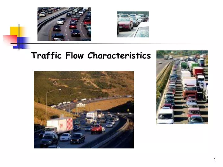
Traffic Flow Characteristics. Traffic Streams. Traffic streams are made up of individual drivers and vehicles, interacting in unique ways with each other and with elements of the roadway and general environment.

E N D
Traffic Streams • Traffic streams are made up of individual drivers and vehicles, interacting in unique ways with each other and with elements of the roadway and general environment. • Because the judgments and abilities of individual drivers come into play, vehicles in the traffic stream do not and cannot behave uniformly. • Further, no two similar traffic streams will behave alike, even under equivalent circumstances, as driver behavior varies with local characteristics and driving habits. • Traffic streams, however, can be described in quantitative terms with the use of some key parameters like volume, speed and density.
Traffic Streams • Traffic facilities are broadly separated into two principal categories: • Uninterrupted flow facilities, and • Interrupted flow facilities • Uninterrupted Flow Facilities are those on which noexternal factors cause periodic interruption to the traffic stream. Example: Freeway • Interrupted Flow Facilities are those having external devices that periodically interrupt traffic flow. Example: Urban Roadways. • The principal devices creating interrupted flow are primarily traffic signal and also STOP and YIELD signs, etc.
Traffic Streams • Uninterrupted and Interrupted Flow are terms that describe the facility and not the quality of flow. • A congested freeway where traffic is almost coming to a halt is still classified as uninterrupted flow facility, because the reason for congestion is internal to the traffic stream. • A well-timed signaling system on an arterial may result in almost uninterrupted traffic flow, but still is classified as interrupted flow facility.
Traffic Stream Parameters • Traffic Stream Parameters fall into two broad categories: • Macroscopic parameters, and • Microscopic parameters. • Macroscopic parameters characterize the traffic stream as a whole • Microscopic parameters characterize the behavior of individual vehicles in the traffic stream with respect to each other.
Traffic Stream Parameters • Macroscopic flow • traffic in the aggregate. • overall speeds, traffic flows, densities, etc. • Microscopic flow • traffic at the level of the individual vehicle • observe the particular behaviors of drivers, and of individual vehicles in the traffic stream. • vehicle headways & lane-changing behavior (merging, diverging, weaving, passing, etc.) critical @ microscopic level.
Traffic Stream Parameters • A traffic stream may be described macroscopically by three parameters: • Volume or Rate of Flow • Speed • Density
Traffic Stream Parameters • Volume and Flow • Volume is defined as the number of vehicles that pass a point on a highway, or a given lane or direction of a highway, during a specified time interval. • Usually expressed as vehicles per unit time, for example, vehicles per hour or vph. • Rate of Flow is the equivalent hourly rate at which vehicles pass a point on a highway lane during a time period less than 1 hour.
Traffic Stream Parameters • Volume and Rate of Flow are two different measures. • Volume is the actual number of vehicles observed or predicted to be passing a point during a given time interval. • Rate of flow represents the number of vehicles passing a point during a time interval less than 1 hour, but expressed as an equivalent hourly rate.
Traffic Stream Parameters • A volume of 200 vehicles observed in a 10-minute period implies a rate of flow of (200 x 60)/10 = 1200 veh/hr. • Note that 1200 vehicles do not pass the point of observation during the study hour, but they do pass the point at that rate for 10 minutes.
Traffic Stream Parameters • Capacity : The maximum number of vehicles per unit time that a particular transportation facility may accommodate (veh/h).
Traffic Stream Parameters • Daily Volumes and Their Use • A common time interval for volumes is a day. • Daily volumes are frequently used as the basis for highway planning and general observations of trends. • Traffic volume projections are often based on measured daily volumes.
Traffic Stream Parameters • Daily Volumes and Their Use (Contd..) • There are four commonly used daily volume parameters: • Average Annual Daily Traffic (AADT): is the average 24-hr traffic volume at a given location over a full 365-day year. • Average Annual Weekday Traffic (AAWT): is the average 24-hr traffic volume occurring on weekdays over a full 365-day year. • Average Daily Traffic (ADT): is an average 24-hr volume at a given location for some period of time less than a year, but more than one day. • Average Weekday Traffic (AWT): is an average 24-hr traffic volume occurring on weekdays for some period less than one year.
Traffic Stream Parameters • Hourly Volumes and Their Use • While daily volumes are useful in highway planning, they cannot be used alone for design or operational analysis purposes. • Traffic volume varies considerably during the course of a 24-hr day. • The single hour of the day that has the highest hourly volume is referred to as the “peak hour”. • Traffic volume within this hour is of greatest interest to traffic engineers in design or operational analysis.
Traffic Stream Parameters • Sub-hourly Volumes and Rates of Flow • The variation within a given hour is also of considerable interest for traffic design and analysis. • The quality of traffic flow is often related to short-term fluctuations in traffic demand. • A facility may have capacity adequate to serve the peak-hour demand, but short-term peaks of flow within the peak hour may exceed capacity, thereby creating a breakdown.
Traffic Stream Parameters • Sub-hourly Volumes and Rates of Flow
Traffic Stream Parameters • Sub-hourly Volumes and Rates of Flow (contd..) • The relationship between hourly volume and the maximum rate of flow within the hour is defined by the Peak Hour Factor (PHF). • where, V = hourly volume, and V15 = maximum 15-minute volume within the hour.
Traffic Stream Parameters • Sub-hourly Volumes and Rates of Flow (contd..) • The maximum value of PHF is 1.00, which occurs when the volume in each 15-min period is equal. • The minimum value is 0.25, which occurs when the entire hourly volume occurs in one 15-min interval. • The normal range of values is between 0.70 and 0.98, with lower values signifying a greater degree of variation in flow during the peak hour.
Traffic Stream Parameters • Speed • Speed is the second principal parameter describing the state of a given traffic stream. • In a moving traffic stream, each vehicle travels at a different speed. • Thus, the traffic stream does not have a single characteristic speed but rather a distribution of individual vehicle speeds. • From the distribution of vehicle speeds, a number of “average” or “typical” values may be used to characterize the traffic stream as a whole.
Traffic Stream Parameters • Speed (contd..) • Average or mean speeds can be computed in two different ways: • Time Mean Speed (TMS) is defined as the average speed of all vehicles passing a point on a highway over some specified time period. • Space Mean Speed (SMS) is defined as the average speed of all vehicles occupying a given section of a highway over some specified time period. • Time mean speed is a point measure, while space mean speed is a measure relating to a length of highway or lane.
Traffic Stream Parameters • Speed (contd..) • where, d is the distance traversed, n is the number of travel times observed and ti is the travel time for i-th vehicle.
Traffic Stream Parameters • Speed (contd..)
Traffic Stream Parameters • Relationship between time mean speed and space mean speed • Time mean speed is greater to equal to space mean speed • The two speeds have the following relationship:
Traffic Stream Parameters • Speed (contd..) • Average Travel Speed and Average Running Speed • They are two forms of space mean speed. • The Average Travel Speed computation uses total average travel time while Average Running Speed computation uses the average running time. • Running time is defined as the time during which the vehicle is in motion while traversing a given highway segment.
Traffic Stream Parameters • Speed (contd..) Example • Consider the case of a 1-mile section of a roadway. On the average, it takes a vehicle 3 minutes to traverse the section, 1 minute of which is stopped time experienced at signalized intersections.
Traffic Stream Parameters • Speed (contd..) • Operating Speed is defined as the maximum safe speed at which a vehicle can be conducted in a given traffic stream, without exceeding the design speed of the highway segment. • Operating speed is difficult to measure. It requires that a test car be driven through the traffic stream in a manner consistent with the definition. • As “maximum safe speed” is a judgmental matter, consistent measurements among test-car drivers are not often achieved.
Traffic Stream Parameters • Density • Density, the third measure of traffic stream conditions, is defined as the number of vehicles occupying a given length of highway or lane. • Usually expressed as vehicles per mile (vpm) or vehicles per mile per lane (vpmpl). • Density is difficult to measure directly, as an elevated point is required.
Traffic Stream Parameters • Density (contd…) • It can, however, be computed from speed and flow rate using the relationship as follows: Where, q = flow rate (vph) vs = space mean speed (mph), and k = density (vpm).
Traffic Stream Parameters • Spacing and Time Headway • Spacing and Time Headway are microscopic measures, because they apply to individual pairs of vehicles within the traffic stream. • Spacing is defined as the distance between successive vehicles in a traffic lane, measured from some common reference point on the vehicles, such as the front bumpers or front wheels. Spacing @ given point
Traffic Stream Parameters • Spacing and Time Headway • Time Headway is the time between successive vehicles as they pass a point along the lane, also measured between common reference points on the vehicles. Particular location
Traffic Stream Parameters • Clearance (ft) = (spacing) – (average vehicle length) • Gap (sec) = (headway) – (time equivalence of the average vehicle length)
Traffic Stream Parameters • Spacing and Time Headway (contd..) • Average values of Spacing and Time Headway are related to the macroscopic parameters as follows: • where, k = density (vpmpl), vs = average speed (ft/sec), q = rate of flow (vphpl), da = average spacing (ft), and ha = average time headway (sec).
Traffic Stream Parameters • Lane occupancy: measure used in freeway surveillance. • Ratio of the time that vehicles are present at a detection station in a traffic lane compared to the observation time.
Traffic Stream Parameters • Lane occupancy • Time that the vehicle used to travel L+C:
Traffic Stream Parameters • Lane occupancy • Assume k vehicles are evenly spread out on 1 mile highway at speed vs mile/hr • Total time needed to have all vehicles pass the detector is: (hrs) • Therefore:
Speed, Flow and Density Relationship • Assume • We have
Properties of speed-density curve • The product of the x-y coordinates of the point P is the flow associated with P • Max flow occurs at:
Properties of speed-flow curve • The slope of the line connecting any point on the curve and the origin is the inverse of the density • Max flow occurred at:
Properties of flow-density curve • The slope of the line connecting any point on the curve and the origin is the space mean speed
General properties for any traffic flow model • Need to satisfy four boundary conditions • Flow is zero at zero density • Flow is zero at maximum density • Mean free-flow speed occurs at zero density • Flow-density curves are convex (i.e. there is a point of max flow)
Connections between speed, density and flow • A: almost zero density, free-flow speed, very low volume • B: increased density, reduced speed, increased volume • C: increased density, reduced speed, max volume • D: jam density, min speed (crawling), very low volume
Traffic Stream Parameters • Since a given flow may occur under two completely different operating conditions (stable and unstable), volume or rate of flow cannot be used as a measure describing the operational quality of the traffic stream. • Speed and density, however, are good measures of the quality of operations, as both uniquely describe the state of the traffic stream.
Macroscopic Models of Traffic Flow • The two most commonly used macroscopic models are: • The Greenshields Model • The Greenberg Model
Macroscopic Models of Traffic FlowGreenshields’ Model • The general model connecting speed, flow, and density discussed so far is a linear model proposed by Greenshield in 1935. • He suggested that the speed and density were linearly related as follows:
Macroscopic Models of Traffic FlowGreenshields’ Model • It can be shown that: • The maximum flow (i.e., capacity) occurs when the speed of the traffic stream is half of the free-flow speed: • The maximum flow (i.e., capacity) occurs when the density is half of the jam density: • The maximum flow, qmax:
Macroscopic Models of Traffic FlowGreenberg’s Model • Greenberg developed a model in 1959, taking speed, flow and density measurements in the Lincoln Tunnel. • Used a fluid-flow analogy concept. • The model is of the following form:
Macroscopic Models of Traffic FlowGreenberg’s Model • It can be shown that: • The maximum flow occurs when speed • The maximum flow occurs when density (k) is related with jam density (kj) as follows: • Then, the maximum flow (qmax) is the product of the density (k) and speed (vs) at maximum flow.
Macroscopic Models of Traffic FlowLimitations of the Models • The Greeshields Model can be used for light or heavy traffic conditions. • The Greenberg Model is useful only for heavy traffic conditions.