Download
1 / 104
1.12k likes | 1.44k Vues
Deterministic Scheduling. Krzysztof Giaro and Adam Nadolski Gdańsk University of Technology. Lecture Plan. Introduction to deterministic scheduling Critical path method Some discrete optimization problems Scheduling to minimize C max Scheduling to minimize C i

E N D
Deterministic Scheduling • Krzysztof Giaro and Adam Nadolski • Gdańsk University of Technology
Lecture Plan • Introduction to deterministic scheduling • Critical path method • Some discrete optimization problems • Scheduling to minimize Cmax • Scheduling to minimize Ci • Scheduling to minimize Lmax • Scheduling to minimize the number of tardy tasks • Scheduling on dedicated processors
Introduction to Deterministic Scheduling Our aim is to schedule the given set of tasks (programs, etc.) on machines (or processors). We have to construct a schedule that fulfils given constraints and minimizes the optimality criterion. Deterministic model:All the parameters of the system and of the tasks are known in advance. • Genesis and practical motivation: • scheduling manufacturing processes, • project planning, • school or conference timetabling, • scheduling processes in multitask operational systems, • distributed computing.
Introduction to Deterministic Scheduling Example 1. Five tasks with processing times p1,...,p5=6,9,4,1,4 have to be processed on three processors to minimize schedule length. Graphical representation of the schedule – Gantt chart • Why the above schedule is feasible? • General constraints in classical scheduling theory: • each task is processed by at most one processor at a time, • each processor is capable of processing at most one task at a time, • other constraints – to be discussed...
Introduction to Deterministic Scheduling Processors characterization • Parallel processors (each processor is capable to process each task): • identical processors – every processor is of the same speed, • uniform processors – processors differ in their speed, but the speed does not depend on the task, • unrelated processors – the speed of the processor depend on the particular task processed. Schedule on three parallel processors
Introduction to Deterministic Scheduling Processors characterization Dedicatedprocessors • Each job consists of the set of tasks preassigned to processors (job Jj consists of tasks Tij preassigned to Pi, of processing time pij). The job is completed at the time the latest task is completed, • some jobs may not need all the processors (empty operations), • no two tasks of the same job can be scheduled in parallel, • a processor is capable to process at most one task at a time. There are three models of scheduling on dedicated processors: • flow shop – all jobs have the same processing order through the machines coincident with machines numbering, • open shop – the sequence of tasks within each job is arbitrary , • job shop – the machine sequence of each job is given and may differ between jobs.
Teachers M1 M2M3 J1 3 2 1 J2 3 2 2 J3 1 1 2 Classes Introduction to Deterministic Scheduling Processors characterization Dedicatedprocessors – open shop (processor sequence is arbitrary for each job). Example. One day school timetable.
Robots M1 M2M3 Ja 3 2 1 Jb 3 2 2 Jc 1 1 2 Details Ja Jb Jc M1 M2 M3 Introduction to Deterministic Scheduling Processors characterization Dedicatedprocessors – flow shop (processor sequence is the same for each job – task Tij must precedeTkj for i<k). Example. Conveyor belt. Dedicated processors will be considered later ...
Introduction to Deterministic Scheduling Tasks characterization There are given: the set of n tasks T={T1,...,Tn} and the set of m machines (processors) M={M1,...,Mm}. • Task Tj : • Processing time. It is independent of processor in the case of identical processors and is denoted pj. In the case of uniform processors, processor Mj speed is denoted bi and the processing time of Tj on Mj is pj/bj. In the case of unrelated processors the processing time of Tj on Mj is pij. • Release (or arrival) timerj. The time at which the task is ready for processing. By default all release times are zero. • Due datedj. Specifies a time limit by which Tj should be completed. Usually, penalty functions are defined in accordance with due dates, or dj denotes the ‘hard’ time limit (deadline) by which Tjmust be completed. • Weightwj – expresses the relative urgency of Tj , by default wj=1.
Introduction to Deterministic Scheduling Tasks characterization • Dependent tasks: • In the task set there are some precedence constraints defined by a precedence relation. TiTj means that task Tj cannot be started until Ti is completed (e.g.Tj needs the results of Ti). • In the case there are no precedence constraints, we say that the tasks are independent (by default). In the other case we say that the tasks are dependent. • The precedence relation is usually represented as a directed graph in which nodes correspond to tasks and arcs represent precedence constraints (task-on-node graph). Transitive arcs are usually removed from precedence graph.
T1 2 T2 T3 T4 3 1 2 T6 T5 4 1 6 T8 T7 2 T10 1 T9 2 Introduction to Deterministic Scheduling Tasks characterization Example. A schedule for 10 dependent tasks (pj given in the nodes).
T1 2 T2 T3 T4 3 1 2 T6 T5 4 1 6 T8 T7 2 T10 1 T9 2 Introduction to Deterministic Scheduling Tasks characterization Example. A schedule for 10 dependent tasks (pj given in the nodes).
Introduction to Deterministic Scheduling Tasks characterization Example. A schedule for 10 dependent tasks (pj given in the nodes). T1 2 T2 T3 T4 3 1 2 T6 T5 4 1 6 T8 T7 2 T10 1 T9 2
Introduction to Deterministic Scheduling Tasks characterization • A schedule can be: • non-preemptive – preempting of any task is not allowed (default), • preemptive – each task may be preempted at any time and restarted later (even on a different processor) with no cost. Preemptive schedule on parallel processors
Introduction to Deterministic Scheduling • Feasible schedule conditions(gathered): • each processor is assigned to at most one task at a time, • each task is processed by at most one machine at a time, • task Tj is processed completely in the time interval [rj,), • precedence constraints are satisfied, • in the case of non-preemptive scheduling no task is preempted, otherwise the number of preemptions is finite.
Introduction to Deterministic Scheduling Optimization criteria • A location of the task Ti within the schedule: • completition timeCi • flow timeFi=Ci–ri, • latenessLi=Ci–di, • tardinessTi=max{Ci–di,0}, • “tardiness flag” Ui=w(Ci>di), i.e. the answer (0/1, yes/no) to the question whether the task is late or not.
Introduction to Deterministic Scheduling Optimization criteria • Most common optimization criteria: • schedule lengthCmax=max{Cj : j=1,...,n}, • sum of completition timesCj = i=1,...,nCi, • mean flow time F = (i=1,...,nFi)/n. Cmax = 9, Cj = 6+9+4+7+8 = 34 A schedule on three parallel processors, p1,...,p5=6,9,4,1,4. • In the case there are tasks weights we can consider: • sum of weighted completition times wjCj = i=1,...,nwiCi, w1,...,w5=1,2,3,1,1 wjCj = 6+18+12+7+8 = 51
Task:T1T2T3 T4 T5 di= 7 7 5 5 8 Some criteria are pair-wise equivalent Li = Ci –di, F= (Ci)/n – (ri)/n. Introduction to Deterministic Scheduling Optimization criteria • Related to due times: • maximum latenessLmax=max{Lj : j=1,...,n}, • maximum tardinessTmax=max{Tj : j=1,...,n}, • total tardinessTj = i=1,...,nTi, • number of tardy tasksUj = i=1,...,nUi, • weighted criteria may be considered, e.g. total weighted tardinesswjTj = i=1,...,nwiTi. Li= –1 2 –1 2 0 Ti= 0 2 0 2 0 Lmax = Tmax = 2 Tj = 4, Uj = 2
Optimization criterion Procession environment Task characteristics Introduction to Deterministic Scheduling Classification of deterministic scheduling problems. | | • is of the form: • P – identical processors • Q – uniform processors • R – unrelated processors • O – open shop • F – flow shop • PF – „permutation” flow shop • J – job shop • Moreover: • there may be specified the number of processors, e.g.O4, • in the case of single processors we just put 1, • we put ‘–’ in the case of processor-free environment.
Introduction to Deterministic Scheduling Classification of deterministic scheduling problems. In the case is empty all tasks characteristics are default: the tasks are non-preemptive, not depended, rj=0, processing times and due dates are arbitrary. • possible values: • pmtn – preemptive tasks, • res – additional resources exist (omitted), • prec – there are precedence constraints, • rj – arrival times differ per task, • pj=1 or UET – all processing times equal to 1 unit, • pij{0,1} or ZUET – all tasks are of unit time or empty (dedicated processors), • Cjdj – dj denote deadlines,
out–tree in–tree Introduction to Deterministic Scheduling Classification of deterministic scheduling problems. • possible values: • in–tree, out–tree, chains ... – reflects the precedence constraints (prec).
Introduction to Deterministic Scheduling Classification of deterministic scheduling problems. Examples. P3|prec|Cmax – scheduling non-preemptive tasks with precedence constraints on three parallel identical processors to minimize schedule length. R|pmtn,prec,ri|Ui – scheduling preemptive dependent tasks with arbitrary ready times and arbitrary due dates on parallel unrelated processors to minimize the number of tardy tasks. 1|ri,Cidi|– – decision problem of existence (no optimization criterion) of schedule of independent tasks with arbitrary ready times and deadlines on a single processor, such that no task is tardy.
Introduction to Deterministic Scheduling Computational complexity theory notations. • Polynomial-time algorithm – an algorithm that runs in at most w(r) steps for every input of size r bits, for some fixed polynomial w. • P (Polynomial) – the set of decision problems that can be solved by a polynomial-time deterministic algorithm. • NP (Non-deterministic Polynomial) – the set of decision problems that can be solved in polynomial time by anon-deterministic algorithm (equivalently: a witness of positive answer can be verified in polynomialtime by a deterministic algorithm). The main hypothesis: P ≠ NP
Reduction – a transformation of one problem A to another problem B, i.e. such a transformation of an input of A into some input of B that the answer toA is affirmative iff the answer toB is affirmative too. Polynomial reduction – a reduction that can be computed in polynomialtime (on deterministic machine). NPC (NP-Complete) – the set of NP problems X such that any other NP problem can be polynomialy reduced to X(i.e. constructing a polynomial-time algorithm solving X would bring the P ≠ NP hypothesis down). Introduction to Deterministic Scheduling Computational complexity theory notations.
Introduction to Deterministic Scheduling Computational complexity theory notations. Some NP-complete problems: • Satisfiability Problem – determine if a given Boolean formula is safisfiable (i.e. there exists such an assignment to the variables that the formula is evaluated to TRUE). • Partition Problem – for a given sequence of positive integers of even sum S verify if it can be partitioned into two subsequences of sums S/2. • Clique Problem– for a given graph G and a positive integer k determine if G contains k-vertex complete subgraph. • Many others...
Introduction to Deterministic Scheduling Computational complexity theory notations. • NPH (NP-Hard) – in practice: optimization versions of NPC problems. • Pseudo-polynomial time algorithm– an algorithm which runs in at most w(r,n1,...,nk) steps for every input of r bits, where ni are the numbers occurring in the input and w is a fixed polynomial. • Strongly NP-hard, NPH! (strongly NP-complete, NPC!) – NP-hard problems (NP-complete problems) that remain NP-hard (NP-complete) evenif all the numbers in the input are bounded by some polynomial of variable r (the size of the input in bits), i.e. believed to be not solvable by any pseudo-polynomial time algorithm.
Introduction to Deterministic Scheduling Input: a sequence A=(a1,...,an) of even sum S. boolean T [0..S/2]; T [0] := true; fors:= 1 to S/2 T [s]:= false; for eachaiA if ( ai≥s ) thenT [s]:= (T [s] or T [s-ai]); end; end; returnT [S/2]; Example. Pseudo-polynomial algorithm for the Partition Problem (dynamic programming), O(nS) complexity: T[s] – the answer to ‘does A contains a subsequence of sum s?’. • Therefore, the Partition Problem is weakly NP-complete. • The Clique Problem is strongly NP-complete (no numbers in the input!)
rj wiFi wiTi wiUi R pi=1 Q Rm Ui Ti F prec Qm P Lmax in–tree out–tree Pm Cmax chain 1 Introduction to Deterministic Scheduling Reductions of scheduling problems
Introduction to Deterministic Scheduling Computational complexity of scheduling problems • If we restrict the number of processors to 1,2,3,, there are 4536 problems: • 416 – polynomial-time solvable, • 3817 – NP–hard, • 303 – open. • How do we cope with NP–hardness? • polynomial-time approximate algorithms with guaranteed approximation ratio, • exact pseudo-polynomial time algorithms, • exact algorithms, efficient only in themean-case, • heuristics (tabu-search, genetic algorithms, etc.), • in the case of small input data – exponential exhaustive search (e.g. branch and bound).
Construct effective algorithm solving X Xd P? Xd NPC? Construct pseudo-polynomial time algorithm for X Xd PseudoP? Xd NPC! ? • Polynomial-time • approximatealgorithms • approximation schemas Yes Do approximations satisfy us? Do not exist No • Small data: exhaustive search (branch & bound) • Heuristics: tabu search, ... Restrict problem X Introduction to Deterministic Task Scheduling General problem analysis schema Optimization problem X decision version Xd
Critical Path Method –|prec|Cmax model consists of a set of dependent tasks of arbitrary lengths, which do not need processors. Our aim is to construct a schedule of minimum length. • Precedence relation is a quasi order in the set of tasks, i.e. it is • anti-reflective: Ti TiTi • transitive Ti,Tj,Tk,(TiTj TjTk) TiTk
Critical Path Method Precedence relation is represented with an acyclicdigraph. • AN (activity on node) network: • nodes correspond to tasks, nodes weights are equal to processing times, • TiTj there exists a directed path connecting node Ti and node Tj, • transitive arcs are removed • AA (activity on arc) network: • arcs correspond to tasks, their length is equal to processing times, • For each node v there exists a path starting at S (source) and terminating at T (sink) passing through v. • TiTj arc Ti end-node is the starting-node of Tj, or there exists a directed path starting at Ti end-node and terminating at Tj start-node. • to construct the network one may need to add apparent tasks – zero-length tasks.
A T3 T1 T T0,p0=0 S T2 T4 B T8,2 T13,6 AN network T4,2 T8,2 T13,6 T4,2 T1,3 T18,5 T1,3 T9,1 T5,4 T14,5 T5,4 T9,1 T14,5 T18,5 T2,8 T10,2 T15,9 T2,8 Example. Translating AN AA we may need to add (zero-length) apparent tasks. T19,3 T10,2 T15,9 T1 T3 T3,2 T6,6 T3,2 T16,6 T6,6 T11,1 T19,3 T11,1 T16,6 T7,9 AA network T17,2 T12,2 T7,9 T2 T4 T12,2 T17,2 D A F I C G S T B E H J Critical Path Method Precedence relation is represented with an acyclicdigraph. Example. Precedence relation for 19 tasks.
Critical Path Method –|prec|Cmax model consists of a set of dependent tasks of arbitrary lengths, which do not need processors. Our aim is to construct a schedule of minimum length. The idea: for every task Ti we find the earliest possible start time l(Ti), i.e. the length of the longest path terminating at that task. How to find these start times? AN network Algorithm : 1. find a topological node ordering (the start of any arc precedes its end), 2. assign l(Ta)=0 for every task Ta without predecessor, 3. assign l(Ti)=max{l(Tj)+pj: exists an arc (Tj,Ti)} to all other tasks in topological order. AN network algorithm: 1. find a topological node ordering, 2. l(S)=0, assign l(v)=max{l(u)+pj: arc Tj connects u and v} to eachnode v, Result:l(Tj) is equal to l(v) of the starting node v of Tj. l(T) is the length of an optimal schedule.
D A F I T8,2 T13,6 T4,2 T18,5 T1,3 T9,1 T5,4 T14,5 C G T2,8 T10,2 T15,9 S T T3,2 T16,6 T6,6 T11,1 T19,3 T17,2 T12,2 T7,9 B E H J Critical Path Method –|prec|Cmax model consists of a set of dependent tasks of arbitrary lengths, which do not need processors. Our aim is to construct a schedule of minimum length. Example. Construction of a schedule for 19 tasks S: A: B: C: D: E: F: G: H: I: J: T: 0 Starting times Topological ordering 3 S:0+3 2 S:0+2 8 S:0+8, A:3+4, B:2+6 A:3+2 5 11 B:2+9 9 C:8+1 ,D:5+2 12 C:8+2, E:11+1 13 E:11+2 F:9+6, G:12+5 17 18 G:12+6, H:13+2 22 I:17+5, J:18+3, G:12+9
S: A: B: C: D: E: F: G: H: I: J: T: 0 3 2 8 5 11 9 12 13 17 18 22 T8,2 T13,6 T4,2 T1,3 T5,4 T9,1 T14,5 T18,5 T2,8 T19,3 T10,2 T15,9 T3,2 T6,6 T11,1 T16,6 T7,9 T12,2 T17,2 D A F I T8,2 T13,6 T4,2 T18,5 T1,3 T9,1 T5,4 T14,5 C G T2,8 T10,2 T15,9 S T T3,2 T16,6 T6,6 T11,1 T19,3 T17,2 T12,2 T7,9 B E H J Critical Path Method
Critical Path Method • Critical Path Method does not only minimize Cmax, but also optimizes all previously defined criteria • We can introduce to the model arbitrary release times by adding for each task Tj extra task of length rj, preceding Tj.
Some Discrete Optimization Problems • maximum flow problem. There is given a loop-free multidigraph D(V,E) where each arc is assigned a capacity c:EN. There are two specified nodes – the source s and the sink t. The aim is to find a flowf:EN{0} of maximum value. • What is a flow of valueF? • eEf(e)c(e), (flows may not exceed capacities) • vV–{s,t} e terminates at vf(e) – e starts at vf(e) = 0, • (the same flows in and flows out for every ‘ordinary’ node) • e terminates at tf(e) – e starts at tf(e) = F, • (F units flows out of the network through the sink) • e terminates at sf(e) – e starts at sf(e) = –F, • (F units flows into the network through the source)
5 1 1 3 2 2 3 2 T S 1 1 4 2 Some Discrete Optimization Problems • maximum flow problem. There is given a loop-free multidigraphD(V,E) where each arc is assigned a capacity c:EN. There are two specified nodes – the source s and the sink t. The aim is to find a flowf:EN{0} of maximum value. Network, arcs capacity
5/2 1/0 1/0 3/2 2/2 2/2 3/1 2/2 T S 1/1 1/1 4/1 2/1 Some Discrete Optimization Problems • maximum flow problem. There is given a loop-free multidigraph D(V,E) where each arc is assigned a capacity c:EN. There are two specified nodes – the source s and the sink t. The aim is to find a flowf:EN{0} of maximum value. ... and maximum flow F=5 Complexity O(|V||E|log(|V|2/|E|)) O(|V|3).
Some Discrete Optimization Problems • Many graph coloring models. • Longest (shortest) path problems. • Linear programming – polynomial-time algorithm known. • The problem of graph matching. There is a given graph G(V,E) with a weight function w:EN{0}. A matching is a subset AE of pair-wise non-neighboring edges. • Maximum matching: find a matching of the maximum possible cardinality ((L(G))). The complexity O(|E||V|1/2). • Heaviest (lightest) matching of a given cardinality. For a given k(L(G)) find a matching of cardinality k and maximum (minimum) possible weight sum. • Heaviest matching. Find a matching of maximum possible weigh sum. The complexity O(|V|3) for bipartite graphs and O(|V|4) in general case.
1 1 1 1 1 1 10 1 10 1 1 1 1 1 1 1 Cardinality: 4 Weight: 4 Cardinality: 3 Weight: 12 Some Discrete Optimization Problems Maximum matching needs not to be the heaviest one and vice-versa.
Scheduling on Parallel Processorsto Minimize the Schedule Length Identical processors, independent tasks Preemptive schedulingP|pmtn|Cmax. McNaughton Algorithm (complexity O(n)) 1. Derive optimal length Cmax*=max{j=1,...,npj/m, max j=1,...,npj}, 2. Schedule the consecutive tasks on the first machine until Cmax* is reached. Then interrupt the processed task (if it is not completed) and continue processing it on the next machine staring at the moment 0. Example.m=3, n=5, p1,...,p5=4,5,2,1,2. i=1,...,5pi=14, max pi=5, Cmax*=max{14/3,5}=5. X* denotes the optimal value (i.e. the minimum possible value) of the parameter X, e.g.Cmax*, Lmax*.
Proof.Partition Problem: there is given a sequence of positive integers a1,...an, such that S=i=1,...,nai. Determine if there exists a sub-sequence of sum S/2? PP P2||Cmax reduction: put n tasks of lengths pj=aj (i=1,...,n) and two processors. Determine if CmaxS/2. Scheduling on Parallel Processorsto Minimize the Schedule Length Identical processors, independent tasks Non-preemptive schedulingP||Cmax. The problem is NP–hard even in the case of two processors (P2||Cmax). There exists an exact pseudo-polynomial dynamic-programming algorithm of complexity O(nCm), for some CCmax*.
Scheduling on Parallel Processorsto Minimize the Schedule Length Identical processors, independent tasks Non-preemptive schedulingP||Cmax. Polynomial-time approximation algorithms. • List Scheduling LS – an algorithm used in numerous problems: • Fix an ordering of the tasks on the list, • Anytime a processor gets free (a task processed by that processor has been completed), schedule the first available task from the list on that processor. In the case of dependent tasks. Task Ti is available if all the tasks Tj it depends of (i.e. TjTi)are completed.
List scheduling Scheduling on Parallel Processorsto Minimize the Schedule Length Identical processors, independent tasks Non-preemptive schedulingP||Cmax. Polynomial-time approximation algorithms. • List Scheduling LS – an algorithm used in numerous problems: • Fix an ordering of the tasks on the list, • Anytime a processor gets free (a task processed by that processor has been completed), schedule the first available task from the list on that processor. Example.m=3, n=5, p1,...,p5=2,2,1,1,3. Optimal scheduling
Proof (includes dependant tasks model P|prec|Cmax). Consider a sequence of tasks T(1),..., T(k) in a LS schedule, such that T(1) – the last completed task, T(2) – the last completed predecessor of T(1)etc. Scheduling on Parallel Processorsto Minimize the Schedule Length Identical processors, independent tasks Non-preemptive schedulingP||Cmax. Polynomial-time approximation algorithms. • List Scheduling LS – an algorithm used in numerous problems: • Fix an ordering of the tasks on the list, • Anytime a processor gets free (a task processed by that processor has been completed), schedule the first available task from the list on that processor. Approximation ratio: LS is 2–approximate: Cmax(LS)(2–m–1)Cmax*. C *max(pmtn) Cmax* Cmax(LS) i=1,...,kp(i)+i pi/m = = (1–1/m)i=1,...,kp(i)+ i pi/m (2–1/m)C *max(pmtn)(2–1/m) Cmax*
Scheduling on Parallel Processorsto Minimize the Schedule Length Identical processors, independent tasks Non-preemptive schedulingP||Cmax. Polynomial-time approximation algorithms. • LPT (Longest Processing Time) scheduling: • List scheduling, where the tasks are sorted innon-decreasing processing times pi order. Approximation ratio. LS is 4/3–aproximate:Cmax(LPT)(4/3–(3m)–1)Cmax*. Unrelated processors, not dependent tasks Preemptive schedulingR|pmtn|Cmax Polynomial time algororihtm – to be discussed later ... • Non-preemptive schedulingR||Cmax • The problem is NP–hard (generalization of P||Cmax). • Subproblem Q|pi=1|Cmax is solvable in polynomial time. • LPT is used in practice.
Scheduling on Parallel Processorsto Minimize the Schedule Length Identical processors, dependent tasks • Preemptive schedulingP|pmtn,prec|Cmax. • The problem is NP–hard. • P2|pmtn,prec|Cmax and P|pmtn,forest|Cmax are solvable in O(n2) time. • The following inequality estimating preemptive, non-preemptive and LS schedules holds • C*max C*(LS) (2–m–1)C*max(pmtn) Proof. The same as in the case of not dependent tasks.
Scheduling on Parallel Processors to Minimize the Schedule Length Identical processors, dependent tasks • Non-preemptive schedulingP|prec|Cmax. • Obviously the problem is NP–hard. • Many unit-time processing time cases are known to be solvable in polynomial time: • P|pi=1,in–forest|Cmax and P|pi=1,out–forest|Cmax (Hu algorithm, complexity O(n)), • P2|pi=1,prec|Cmax (Coffman–Graham algorithm, complexity O(n2)), • Even P|pi=1,opositing–forest|Cmax i P2|pi{1,2},prec|Cmax are NP–hard. • Hu algorithm: • out–forest in–forest reduction: reverse the precedence relation. Solve the problem and reverse the obtained schedule. • in–forestin–tree: add extra task dependent of all the roots. After obtaining the solution, remove this node from the schedule. • Hu algorithm sketch: list scheduling for dependent tasks + descending distance from the root order.