Download
1 / 25
250 likes | 355 Vues
Graph Sparsifiers. Nick Harvey University of British Columbia Based on joint work with Isaac Fung, and independent work of Ramesh Hariharan & Debmalya Panigrahi. TexPoint fonts used in EMF. Read the TexPoint manual before you delete this box.: A A A.

E N D
Graph Sparsifiers Nick Harvey University of British Columbia Based on joint work with Isaac Fung,and independent work of RameshHariharan & DebmalyaPanigrahi TexPoint fonts used in EMF. Read the TexPoint manual before you delete this box.: AAA
Approximating Dense Objectsby Sparse Objects • Floor joists Wood Joists Engineered Joists
Approximating Dense Objectsby Sparse Objects • Bridges Masonry Arch Truss Arch
Approximating Dense Objectsby Sparse Objects • Bones Human Femur Robin Bone
Approximating Dense Objectsby Sparse Objects • Graphs Dense Graph Sparse Graph
Cut Sparsifiers Graph Sparsifiers (Karger ‘94) • Weighted subgraphs that approximately preserve graph structure • Input: Undirected graph G=(V,E), weights u : E !R+ • Output: A subgraphH=(V,F) of G with weightsw : F!R+ such that |F| is small and u(±G(U)) = (1§²) w(±H(U)) 8UµV weight of edges between U and V\U in G weight of edges between U and V\U in H G H
Spectral Sparsifiers (Spielman-Teng ‘04) • Weighted subgraphs that approximately preserve graph structure • Input: Undirected graph G=(V,E), weights u : E !R+ • Output: A subgraphH=(V,F) of G with weightsw : F!R+ such that |F| is small and xTLGx = (1 §²) xTLHx 8x2RV Laplacian matrix of G Laplacian matrix of H G H
Motivation:Faster Algorithms Algorithm A for some problem P Dense Input graph G Exact/Approx Output Min s-t cut, Sparsest cut,Max cut, … (Fast) Sparsification Algorithm Algorithm Aruns faster on sparse input Sparse graph H Approximatelypreserves solution of P Approximate Output
State of the art n = # vertices m = # edges c = large constant ~ *: The best algorithm in our paper is due to Panigrahi.
Random Sampling Eliminate most of these • Can’t sample edges with same probability! • Idea: [Benczur-Karger ’96]Sample low-connectivity edges with high probability, and high-connectivity edges with low probability Keep this
Generic algorithm [Benczur-Karger ‘96] • Input: Graph G=(V,E), weights u : E !R+ • Output: A subgraph H=(V,F) with weights w : F!R+ • Choose ½ (= #sampling iterations) • Choose probabilities { pe:e2E} • For i=1 to ½ • For each edge e2E • With probability pe Add e to F Increase we by ue/(½pe) How should we choosethese parameters? • E[|F|]·½¢epe • E[ we ] = ue8e2E • ) For every UµV, E[ w(±H(U)) ] = u(±G(U)) Goal 1: E[|F|] = O(n log n / ²2) Goal 2: w(±H(U)) is highly concentrated
Benczur-Karger Algorithm • Input: Graph G=(V,E), weights u : E !R+ • Output: A subgraph H=(V,F) with weights w : F!R+ • Choose ½ = O(log n /²2) • Let pe = 1/“strength” of edge e • For i=1 to ½ • For each edge e2E • With probability pe Add e to F Increase we by ue/(½pe) “strength” is a slightly unusual quantity, but Fact 3:Can estimate all edge strengths inO(m log3 n) time “strength” is a slightly unusual quantity Question:[BK ‘02]Can we use connectivity instead of strength? • Fact 1: E[|F|] = O(n log n / ²2) • Fact 2: w(±H(U)) is very highly concentrated • ) For every UµV, w(±H(U)) = (1 §²) u(±G(U))
Our Algorithm • Input: Graph G=(V,E), weights u : E !R+ • Output: A subgraph H=(V,F) with weights w : F!R+ • Choose ½ = O(log2 n /²2) • Let pe = 1/“connectivity” of e • For i=1 to ½ • For each edge e2E • With probability pe Add e to F Increase we by ue/(½pe) • Fact 1: E[|F|] = O(n log2 n / ²2) • Fact 2: w(±H(U)) is very highly concentrated • ) For every UµV, w(±H(U)) = (1 §²) u(±G(U)) • Extra trick:Can shrink |F| to O(n log n / ²2) by using Benczur-Karger to sparsify our sparsifier!
Motivation for our algorithm Connectivities are simpler and more natural ) Faster to compute Fact:Can estimate all edge connectivitiesin O(m + n log n) time [Ibaraki-Nagamochi ’92] ) Useful in other scenarios Our sampling method has been used to compute sparsifiers in the streaming model [Ahn-Guha-McGregor ’12]
Overview of Analysis Most Cuts are Big & Easy! Most cuts hit a huge number of edges) extremely concentrated )whp, most cuts are close to their mean
Overview of Analysis Hits only one red edge) poorly concentrated Hits many red edges) reasonably concentrated Low samplingprobability High connectivity There are few small cuts [Karger ’94], so probably all are concentrated. Key Question:Are there few such cuts? Key Lemma: Yes! The same cut also hits many green edges) highly concentrated This masks the poor concentration above High samplingprobability Low connectivity
Notation: kuv = min size of a cut separating u and v • Main ideas: • Partition edges into connectivity classesE = E1[E2[ ... Elog nwhere Ei = { e : 2i-1·ke<2i } • Prove weight of sampled edges that each cuttakes from each connectivity class is about right • This yields a sparsifier U
Prove weight of sampled edges that each cuttakes from each connectivity class is about right • Notation: • C = ±(U) is a cut • Ci:= ±(U) ÅEi is a cut-induced set • Chernoff bounds can analyze each cut-induced set, but… • Key Question: Are there few small cut-induced sets? C2 C3 C1 C4
Counting Small Cuts • Lemma: [Karger ’93] Let G=(V,E) be a graph. Let K be the edge-connectivity of G. (i.e., global min cut value) Then, for every ®¸1,|{ ±(U) : |±(U)|·®K }| < n2®. • Example: Let G = n-cycle. Edge connectivity is K=2. Number of cuts of size c = £( nc ).)|{ ±(U) : |±(U)|·®K }| ·O(n2®).
Counting Small Cut-Induced Sets • Our Lemma:Let G=(V,E) be a graph. Fix any BµE. Suppose ke¸K for all e in B. (kuv = min size of a cut separating u and v) Then, for every ®¸1,|{ ±(U) ÅB : |±(U)|·®K }| < n2®. • Karger’s Lemma:the special case B=E and K=min cut.
When is Karger’sLemma Weak? • Lemma: [Karger ’93] Let G=(V,E) be a graph. Let K be the edge-connectivity of G. (i.e., global min cut value) Then, for every c¸K,|{ ±(U) : |±(U)|·c }| < n2c/K. ² • Example: Let G = n-cycle. • Edge connectivity is K=2 • |{ cuts of size c}| < nc K = ² < n2c/²
Our Lemma Still Works • Our Lemma:Let G=(V,E) be a graph. Fix any BµE. Suppose ke¸K for all e in B. (kuv = min size of a cut separating u and v) Then, for every ®¸1,|{ ±(U) ÅB : |±(U)|·®K }| < n2®. ² • Example: Let G = n-cycle. • Let B = cycle edges. • We can take K=2. • So |{ ±(U) ÅB : |±(U)|·®K }| < n2®. • |{cut-induced subsets of B induced by cuts of size · c}|·nc
Algorithm for Finding a Min Cut[Karger ’93] • Input: A graph • Output: A minimum cut (maybe) • While graph has 2 vertices • Pick an edge at random • Contract it • End While • Output remaining edges • Claim: For any min cut, this algorithm outputs it with probability ¸ 1/n2. • Corollary: There are · n2 min cuts.
Splitting Off Replace edges {u,v} and {u’,v} with {u,u’}while preserving edge-connectivity between all vertices other than v Finding a Small Cut-Induced Set v v u u u’ u’ • Input: A graph G=(V,E), and BµE • Output: A cut-induced subset of B • While graph has 2 vertices • If some vertex v has no incident edges in B • Split-off all edges at v and delete v • Pick an edge at random • Contract it • End While • Output remaining edges in B Wolfgang Mader • Claim: For any min cut-induced subset of B, this algorithm outputs it with probability >1/n2. • Corollary: There are <n2 min cut-induced subsets of B
Conclusions • Sampling according to connectivities gives a sparsifier • We generalize Karger’s cut counting lemma Questions • Improve O(log2 n) to O(log n) in sampling analysis • Applications of our cut-counting lemma?