Download
1 / 2
20 likes | 115 Vues
The visibility of Venus. Albert J. Ahumada ( al.ahumada@nasa.gov ) NASA Ames Research Center . A Digital Venus

E N D
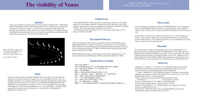
The visibility of Venus Albert J. Ahumada (al.ahumada@nasa.gov) NASA Ames Research Center A Digital Venus Following Westheimer's (1985) suggestion for representing a point source on a digital display, we set the display resolution to 120 pixels per degree and solve for the contrast needed to represent Venus. Using a sky luminance measurement of 4200 cd/m^2 (Minolta CS100A) , the required single pixel contrast turns out to be 2.22. The assuming an effective duration of 0.25 sec, the contrast energy relative to 10^-3 degree^2 seconds is 19.3 dBB. Observations On a clear sunny day, September 10, 2010, at 2:00 PM (PDT), three of the 16 Modelfest observers (ABW, BRB, CVR) looked for Venus, using the Moon as a guide. BRB was unable to locate it, but the other two and two other staff (AJA, BDA) were able to keep it in view. It takes minutes to find, but once found it is easy to keep in view. It does not appear to flicker or vary in contrast. When you look away and then look back, it can take many seconds to find it again. It is the smallest object I have ever seen (smaller than you expect before you find it). It looks round and white. Abstract Venus is the only planet or star that can be seen by the naked eye during the day. Following the method of Westheimer (1985) for representing a point source as a single pixel on a screen with a resolution of 120 pixels per degree, we can convert the magnitude of Venus and the sky luminance into a luminance contrast signal with a contrast of 2.22. Detection models calibrated to the Modelfest data predict that such a target is below threshold (Watson and Ahumada, 2005). Modifications are proposed to the models to keep Venus visible. The Standard Observer Watson and Ahumada (2005) propose a single filter model fit to the Modelfest data as a Spatial Standard Observer model for small target contrast detection. The recommended model which has an exponentiated hypersecant high spatial frequency response predicts an 83 per cent detection threshold of 22.1 dBB. The DoG contrast sensitivity energy model predicts a threshold of 23.8 dBB. When the high spatial frequency cutoff parameter of the DoG is changed from 15 to 25 cycles per degree (Liang & Westheimer, 1995) the predicted threshold is 19.3 dBB. Discussion The possible need for a higher spatial frequency response for a Standard Observer as arisen before (Watson & Ahumada, 2008). The Standard Observer (7.2 dBB) misses the median Modelfest threshold (5.5 dBB) for the sigma = 1.05 arc min Gaussian. The amount is smaller, but the spots suffer from spatial uncertainty relative to the multitude of 4 cpd Gabors (Ahumada, Scharff, & Watson, 2007). More modeling is needed for the processes by which the visual system acquires and tracks small targets as they flit about the retina. Figure 1. The phases of Venus. At its closest approach, Venus subtends 66 arc seconds. (credit: TBGS Observatory, photo by Chris Proctor; http://venus.aeronomie.be/ en/venus/phasesvenus.htm Standard Observer Model function dBthr = ... sso(csftype,beta_is_2,pixperdeg,contrast_image) im = contrast_image; n = size(im,1) ; ppd = pixperdeg; parm = get_parms(csftype,beta_is_2); gain = parm(4); beta = parm(8); s = parm(10); csf = get_csf(n,parm,csftype,ppd) ; csf = csf.*oblique2d(n,ppd); im = real(ifft2(fft2(im).*csf)) ; im = im.*gauss2(n, s*ppd) ; dBthr = -20*log10(norm(im(:),beta)*gain/ppd^(2/beta)) ; References Ahumada, A. J., Scharff, L. V. S., Watson, A. B. (2007) What Image Does the Visual System Detect Best? Vision Sciences Society Annual Meeting, May, Sarasota, FL, http://vision.arc.nasa.gov/personnel/al/talks/07vss/07vssSlides.pdf Liang, J., Westheimer, G. (1995) Optical performances of human eyes derived from double-pass measurements. Journal of the Optical Society of America A 12, 1411-1416. Modelfest http://vision.arc.nasa.gov/modelfest/. NASA http://nssdc.gsfc.nasa.gov/planetary/factsheet/venusfact.html Venus Phases http://venus.aeronomie.be/en/venus/phasesvenus.htm Watson, A. B & Ahumada, A. J. Jr. (2005)). A standard model for foveal detection of spatial contrast. Journal of Vision 5, 717-740. Watson, A. B & Ahumada, A. J. Jr. (2008) Predicting visual acuity from wavefront aberrations, Journal of Vision 8 (4), http://journalofvision.org/8/4/17/. Westheimer, G. (1985 )The oscilloscopic view: retinal illuminance and contrast of point and line targets. Vision Research 25:1097–103. Venus Venus has a nearly circular (eccentricity of 0.0067) orbit with a radius of 0.72 AU (the mean distance from the Earth to the Sun) in a plane close to that of the Earth's orbit (3.39 deg). Its brightness (illuminance) is a function of the distances and angles among the three bodies and is essentially periodic (synodic period = 584 days). Its Standard Visual Magnitude M(0,1) (the illuminance seen from the Sun at a distance of 1 AU) is -4.40 (a magnitude of 0 corresponds to an illumination of 2.54E-6 lux and a magnitude of 1 is -0.4 log units higher). Using the circular, coplanar theory to interpolate the illuminance cycle, the estimated visual magnitude on September 10, 2010 was -4.74.
Standard Observer Model Subroutines function filt = oblique2d(n,ppd) gamma = 3.48 *(n/ppd); % cycles per image lambda = 13.57 *(n/ppd); f1 = repmat(fltf1(n),[n 1]) ; % fx theta = atan2(f1',f1); filt = min(1,exp(-(fltf2(n)-gamma)/lambda)) ; filt = 1-(1-filt) .*sin(2*theta).^2 ; function g = gauss2(n,s) % n must be even g1 = exp(-(([1:n]-n/2)/s).^2); g = g1'*g1; Standard Observer Model CSF function csf = get_csf(n,parm,csftype,ppd) f0 = n*parm(2)/ppd; f1 = n*parm(3)/ppd; a = parm(4); p = parm(6); switch csftype case 1; csf = fltsechp2( n, f0, p)- a*fltsech2( n, f1); % HPmH case 2; csf = fltsechp2( n, f0, p)- a*filtgaus2(n,f1); % HPmG case 3; csf = fltyqm2( n, f0, f1, a); % YQM case 4; csf = fltexp2( n, f0)- a*filtgaus2(n,f1); % EmG case 5; csf = fltexp2( n, f0)- a*filtgaus2(n,f1); % LP case 6; csf = fltsech2( n, f0)- a*filtgaus2(n,f1); % HmG case 7; csf = fltsech2( n, f0)- a*fltsech2( n, f1); % HmH case 8; csf = fltms2( n, f0, a, p); % MS otherwise; csf = filtgaus2(n,f0)- a*filtgaus2(n,f1); % DoG end function f = fltf1( n) n2 = floor(n/2); f = [[0:ceil(n/2)-1] [0:n2-1]-n2]; function filter = fltgaus1( n, f) filter = fltf1(n)/f; filter = exp(-(filter.*filter)) ; function flt = filtgaus2(n, f) flt1 = fltgaus1(n,f); flt=flt1'*flt1; function f = fltf2(n) f1 = fltf1(n); f = repmat(f1,[n 1]) ; % fx f = f.*f ; % fx^2 f = sqrt(f + f') ; % sqrt(fx^2 + fy^2) function filter = fltsechp2( n, f, p) filter = sech((fltf2(n)/f).^p) ; function filter = fltexp2( n, f) filter = exp(-fltf2(n)/f) ; function filter = fltms2( n, f, a, p) filter = fltf2(n)/f; filter = exp(-filter.^p)*(1 - a + filter) ; function filter = fltyqm2( n, f0, f1, a) filter = fltf2(n)/f0; filter = exp(-filter)./(1 + a./(1+filter*(f0/f1))) ; Magnitude Interpolation by Days function mag = venusmag(day) % Venus magnitude assuming flat, circular orbits % of Earth and Venus % Problem: what are a and dve as a function of the % 583.92 day synodic period % Tropical orbit periods (days) 224.695 365.242 delv = 2*pi/224.695 ; % radians per day dele = 2*pi/365.242 ; dvsr = 108.25/149.6 ; % 0.7236 day = [0:584]; xe = sin(dele*day); ye = -cos(dele*day) ; xv = -dvsr*sin(delv*day); yv= dvsr*cos(delv*day) ; dver = sqrt((xv - xe).^2 + (yv - ye).^2) ; a = acos((dver.^2 + dvsr^2 -1)./(2*dver*dvsr) ); p = (1-a/pi).*cos(a) + (1/pi)*sin(a) ; % p(a)/p(0) mag = -4.40 + 2.5*log10(1./p) + 5*log10(dvsr*dver) ; Standard Observer Model Parameters function parm = get_parms(csftype,beta_is_2) parms = zeros(9,7,2); parms(:,:,1) = [ ...% Gain f0 f1 a beta p s 373.08 4.1726 1.3625 0.8493 2.4081 0.7786 0.6273 289.45 5.3459 1.9793 0.7983 2.4054 0.8609 0.6311 466.38 7.0629 0.6951 7.7712 2.3557 0 0.5790 360.24 7.5237 1.8972 0.8155 2.4725 0 0.7071 214.46 3.2316 0 0.7127 2.4902 0.8081 0.7118 258.17 6.8432 1.7483 0.7778 2.3277 0 0.5579 271.71 6.7770 1.0461 0.8082 2.2950 0 0.5311 551.29 1.7377 0 1.0465 2.3643 0.6937 0.5702 272.74 15.3870 1.3456 0.7622 1.9960 0 0.3548] ; parms(:,:,2) = [ ...% Gain f0 f1 a beta p s 501.20 4.3469 1.4476 0.8514 2 0.7929 0.3652 359.87 6.0728 1.9505 0.7931 2 0.9186 0.3655 621.38 7.0856 0.7285 8.0721 2 0 0.3656 504.43 7.6399 1.9788 0.8163 2 0 0.3635 299.21 3.3578 0 0.7193 2 0.8009 0.3612 329.93 6.9248 1.8045 0.7827 2 0 0.3662 345.78 6.7581 1.1210 0.8128 2 0.7748 0.3596 271.70 15.3852 1.3412 0.7615 2 0 0.3563]; parm = parms(csftype,:,1+beta_is_2); Acknowledgements Supported by NASA Space Human Factors Engineering and the U.S. Navy.