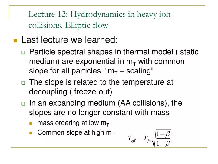
Lecture 12: Hydrodynamics in heavy ion collisions. Elliptic flow

1. Lecture 12: Hydrodynamics in heavy ion collisions. Elliptic flow • Last lecture we learned: • Particle spectral shapes in thermal model ( static medium) are exponential in mT with common slope for all particles. “mT – scaling” • The slope is related to the temperature at decoupling ( freeze-out) • In an expanding medium (AA collisions), the slopes are no longer constant with mass • mass ordering at low mT • Common slope at high mT

2. Hydrodynamics inspired parameterization Obtain from fit: Flow velocity Freeze-out temperature “blast wave” fits to spectra Retiere and Lisa – nucl-th/0312024 PHENIX - Phys. Rev. C 69, 034909 (2004)

3. Today: • Introduce a new observable ( elliptic flow) sensitive to the early stage of the collisions • More about how hydrodynamics works and what we learn from it

4. PHOBOS z Paddle signal Peripheral Collision: Central Collision y x  Small number of participating nucleons  Large Npart The Geometry of a Heavy Ion Collision Npart Participantsthat undergo Ncoll Collisions A-0.5Npart Spectators A-0.5Npart Spectators …and we can measure this!  We can classify collisions according to centrality.

5. f 2v2 State of Matter appears strongly interacting (Similar to a “fluid”) “elliptic flow” • Experiment finds a clear v2 signal • If system was freely streaming the spatial anisotropy would be lost

6. Basics of Hydrodynamics Hydrodynamic Equations Energy-momentum conservation Charge conservations (baryon, strangeness, etc…) Need equation of state (EoS) P(e,nB) to close the system of eqs.  Hydro can be connected directly with lattice QCD For perfect fluids (neglecting viscosity), Energy density Pressure 4-velocity Within ideal hydrodynamics, pressure gradient dP/dx is the driving force of collective flow.  Collective flow is believed to reflect information about EoS!  Phenomenon which connects 1st principle with experiment Caveat:Thermalization,l << (typical system size)

7. Inputs to Hydrodynamics Final stage: Free streaming particles  Need decoupling prescription t Intermediate stage: Hydrodynamics can be valid if thermalization is achieved.  Need EoS z • Initial stage: • Particle production and • pre-thermalization • beyond hydrodynamics • Instead, initial conditions for hydro simulations Need modeling (1) EoS, (2) Initial cond., and (3) Decoupling

8. Initial conditions • Hydro requires thermal equilibrium ( at least locally) • Thus, the initial thermalization stage in a heavy ion collision lies outside the domain of applicability of the hydrodynamic approach and must be replaced by initial conditions for the hydrodynamic evolution. • Different approaches explored: • treat the two colliding nuclei as two interpenetrating cold fluids feeding a third hot fluid in the reaction center (“three-fluid dynamics”). This requires modelling the source and loss terms describing the exchange of energy, momentum and baryon number among the fluids. • microscopic transport models: (parton cascades) VNI, VNI/BMS, MPC, AMPT estimate the initial energy and entropy distributions in the collision region before switching to a hydrodynamic evolution. However the thermalization mechanism is still poorly understood at a microscopic level

9. Initial conditions ( continued) • Assuming • isentropic expansion • Particle multiplicities in the final state ( measured) define the entropy • Need to go from: measured final multiplicity to initial distribution of energy density • Use Glauber model to predict Npart and Ncoll for a given impact parameter • Density distribution of the nucleus • Integrate along the path of each nucleon to get the nuclear thickness function and Npart, Ncoll

10. The initial entropy density and energy density is taken proportional to the a*Npart +b*Ncoll Initial conditions

11. EoS • EoS can either be modeled or extracted from lattice QCD calculations. • Typically – modeled • low temperature regime: non-interacting hadron gas with (smallish) speed of sound cs2= ∂p/∂e ≈ 0.15 • Above the transition: free gas of massless quarks and gluons: cs2= ∂p/∂e = 1/3

12. Decoupling • hydrodynamic description begins to break down again once the transverse expansion becomes so rapid and the matter density so dilute that local thermal equilibrium can no longer be maintained. • Rely on the fact that the entropy density, energy density, particle density and temperature profiles are directly related and all have similar shapes. Thus, decouple on a surface of constant temperature and convert the fluid cells to particles • “Sudden freeze-out” goes from 0 mean free path to infinite mean free path – artificial • Better method: a hybrid approach. After converting to particles – hand the output to a microscopic model that will allow for more re-scattering and a natural freeze-out when matter gets very dilute

13. PFK, J. Sollfrank, U. Heinz, PRC 62 (2000) 054909 Time evolution of anisotropies Coordinate space Momentum space Geometry converts to Momentum Space

14. Kolb, et al STAR Collective effect probes equation of state Hydrodynamics can reproduce magnitude of elliptic flow for p, p. BUT correct mass dependence requires QGP EOS!! NB: these calculations have viscosity = 0 and 1s order phase transition. We have concluded that medium behaves as an ideal liquid.

15. Hydro. Calculations Huovinen, P. Kolb, U. Heinz STAR v2 reproduced by hydrodynamics PRL 86 (2001) 402 central • see a large pressure buildup • anisotropy  happens fast while system is deformed • success of hydrodynamics early equilibration ! • ~ 0.6 fm/c

16. Eccentricity scaling in hydrodynamics Eccentricity scaling observed in hydrodynamic model over a broad range of centralities Bhalerao, Blaizot, Borghini, Ollitrault , nucl-th/0508009 R: measure of size of system

17. Eccentricity scaling in data k~3.1 Cu has a smaller nuclear radius than Au, Hence, Cu+Cu collisions produce a smaller system than Au+Au for the same centrality • v2 scales with eccentricity • for different centralities and different colliding systems • Indicative of high degree of thermalization

18. Estimation of cs Equation of state for a relativistic pion gas: relation between pressure and energy density v2/ε for <pT> ~ 0.45 GeV/c (obtained from pT spectra) • cs ~ 0.35 ±0.05, (cs2 ~ 0.12), soft EOS • The matter does not spend a large amount of time in a mixed phase, indicating a weak first order phase transition or cross-over

19. Excitation function of v2: data vs theory

20. proton pion v2 -AND- spectra nucl-ex/0410003 • Not all hydro models work • Need to model • dissipative effects • in the hadron gas • stage to reproduce • simultaneously • v2 and spectra

21. Where else does hydro fail ? • In most early hydro calculations: boost invariance is assumed • This simplifies a lot the hydro equations, because you don’t need to solve them in 3D , but rather 2D +time • You pay the price that the calculations do not reproduce the v2 data a a function of rapidity

22. What have we learned from v2 data where hydro does work ? Very rapid thermalization is required Very small viscosity Next ask: what are the quanta that flow ?

23. Scaling v2 with transverse kinetic energy Scaling breaks Baryons scale together Mesons scale together Scaling holds up to ~1 GeV • KET scaling is can be viewed as hydrodynamic scaling • Matter behaves hydrodynamically for KET≤ 1 GeV • Hint of partonic degrees of freedom at higher KET

24. Test for partonic degrees of freedom KET/n gives kinetic energy per quark, assuming that each quark carries equal fraction of kinetic energy of hadron Scaling holds over the whole range of KET and is comprehensive

25. Kinetic energy scaling: centrality dependence • KET scaling breaks at lower KET for more peripheral collisions • KET/n scaling holds across the whole KET range for centralities presented • KET scaling provides a link between hydrodynamic and recombination mechanisms in the development of flow

27. Methods to measure elliptic flow

28. Two-particle correlation method in PHENIX Au+Au √s=130 GeV Correlation function is fitted with a functional a(1+2v2 cos(2ΔΦ) ), from which v2 is extracted, a is a normalization constant

29. Two-particle correlation methods Fixed pT method Assorted pT method 2 correlation functions Divide red by sqrt(green) Get v2’ pT pT

30. Cumulant Method Two-particle correlations can be decomposed into a term containing correlations with the reaction plane (flow) and a term corresponding to direct correlations between the particles (non-flow): cumulant method Borghini, Dinh and Ollitrault (Phys.Rev.C 64 054901 (2001)) allows for detailed integral and differential measurements of v2. In this method, flow harmonics are calculated via the cumulants of multiparticle azimuthal correlations and non-flow contributions are removed by higher order cumulants. The second order cumulant is defined as: The second term is due to direct correlations between two particles, which may be due to quantum correlations, momentum conservation, jets, etc.

31. Azimuthal anisotropy from multi-particle correlations If flow predominates, cumulants of higher order can be used to reduce non-flow contributions • Following the decomposition strategy presented earlier for two-particle correlations, the 4 particle correlations can be similarly decomposed as follows: Two-particle non-flow contributions removed

32. Comparison of v2 obtained from different methods • Three different methods applied in PHENIX • RP and cumulant method applied in STAR • They agree within errors for Au+Au collisions for low pT

33. Do we have other handles on cs ? What happens to a fast parton moving through the medium? one idea is that it might generate a shock wave and emit radiation at a characteristic angle that depends on cs (the speed of sound in the medium) ... or, that there would be Cerenkov radiation of gluons ... or, that it is deflected in the dense, flowing medium Casalderrey-Solana, Shuryak and Teaney, hep-ph/0411315 Koch, Majumder, X.-N. Wang, nucl-th/0507063

34. Jet shape vs centrality PHENIX preliminary J. Jia

35. Jet shape vs centrality PHENIX preliminary J. Jia

36. D D Jet shape vs centrality PHENIX preliminary J. Jia Near side : broadening, Away side: splitting

37. Pair opening angle Trigger particle Cherenkov cones? Mach cones? Suggestive of…

38. The medium (“fluid”) appears to have low viscosity • Same phenomena observed in gases of strongly interacting atoms (Li6) From R. Seto M. Gehm, et alScience 298 2179 (2002) strongly coupled viscosity=0 weakly coupled finite viscosity The RHIC fluid behaves like this, that is, viscocity~0

39. State of Matter appears strongly interacting (Similar to a “fluid”) Once again, in Pictures, what we see in experiment… • Initial spatial anisotropy converted into momentum anisotropy (think of pressure gradients…) • Efficiency of conversion depends on the properties of the medium • In particular, the conversion efficiency depends on viscosity Pictures from: M. Gehm, et al., Science 298 2179 (2002)