Hashing

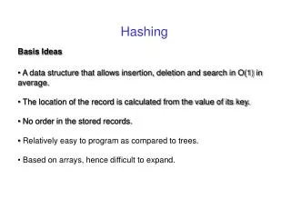
1. Hashing • Basis Ideas • A data structure that allows insertion, deletion and search in O(1) in average. • The location of the record is calculated from the value of its key. • No order in the stored records. • Relatively easy to program as compared to trees. • Based on arrays, hence difficult to expand.

2. …Basic ideas • Consider records with integer key values: • 0, 1, 2, 3, 4, 5, 6, 7, 8, 9 • Create a table of 10 cells: index of each cell in the range [0..9]. • Each record is stored in the cell whose index corresponds to its key value. key: 2 … … key: 8 … … • Need to compress the huge range of numbers. Use of a hash function. • It hashes a number in a large range into a number in a smaller range, corresponding to the index numbers in an array.

3. Definitions • Hashing • The process of accessing a record, stored in a table, by mapping the value of its key to a position in the table. • Hash function • A function that maps key values to table positions. • Hash table • The array where the records are stored. • Hash value • The value returned by the hash function. It usually corresponds to a position in the hash table.

4. Perfect hashing Hash table Key 2 Hash function: Key … … 8 H(key) = key Record Key 8

5. …Perfect hashing • Each key value maps to a different position in the table. • All the keys need to be known before the table is created. • Problem: what if the keys are neither contiguous nor in the range of the indices of the table? • Solution: find a hash function that allows perfect hashing! Is this always possible?

6. Example: • A company has 100 employees. Social Insurance Number (SIN) is used as a key for a each record. • Given a 9 digits SIN, should we create a table of 1,000,000,000 cells for only 100 employees? • Knowing the SI Numbers of all 100 employees in advance does not guarantee to find a perfect hash function.

7. The birthday paradox: • what is the number of persons that need to be together in a room in order to, “most likely”, have two of them with the same date of birth (month/day)? • Answer: only 23 people. • Hint: calculate p the probability that two persons have the same date of birth. • 1 - 364/365 · 363/365 · 362/365 · … · (365 - n + 1)/365 • if N = 365 and there are 23 records to hash • the probability of having at least one collision is… 0.5063! • => It is easy to have identical value using a Random distribution. It is difficult to conceive a good hashing function. • Hash functions that allow perfect hashing are so rare that it is worth looking for them only in special circumstances. • In addition, it is often that the collection of records is not known in advance.

8. Collisions • What if we cannot find a perfect hash function? • Collision: more than one key will map to the same location in the table! • Can we avoid collisions? No, except in the case of perfect hashing (rare). • Solution: select a “good” hash function and use a collision-resolution strategy. • A good hash function: • The hash function, h, must be computationally simple • It must distribute keys evenly in the address space

9. Example of collision: • The keys are integers and the hash function is: • hashValue = keymod tableSize • If tableSize = 10, all records whose keys have the same rightmost digit have the same hash value. Insert 13 and 23 23

10. A poor hash function: • Maps keys non-uniformly into table locations, or maps a set of contiguous keys into clusters. • An ideal hash function: • Maps keys uniformly and randomly onto the entire range of table locations. • Each location is equally likely to be used for a randomly chosen key. • Fast computation.

11. To build a hash function: • We will generally assume that the keys are the set of natural integer numbers N = {0, 1, 2, ……}. • If they are not, then we can suitably interpret them to be natural numbers. • Mapping: • For example, a string over the set of ASCII characters, can be interpreted as an integer in base 128. • Consider key = “data” • hashValue = (‘a’+’t’×128+’a’ ×1282+’d’ ×1283) modtableSize

12. This method generates huge numbers that the machine might not store correctly. • Goal: reduce the number of arithmetic operations and generate relatively small numbers. • Solution: Compute the hash value in several step using each time the modulo operation. • hashValue = ‘d’ modtableSize • hashValue = (hashValue×128 + ‘a’) modtableSize • hashValue = (hashValue×128 + ‘t’) modtableSize • hashValue = (hashValue×128 + ‘a’) modtableSize

13. Hash function : division • H(key) = keymodtableSize • 0 ≤ keymodtableSize ≤ tableSize-1 • Empirical studies have shown that this function gives very good results. • Assume H(key) = keymodtableSize • All keys such that key mod tableSize = 0 map into position 0 in the table. • All keys such that key mod tableSize = 1 map into position 1 in the table. • This phenomenon is not a problem for position 0 and 1, but…

14. Assume tableSize = 25 • All keys that are multiples of 5 will map into positions 0, 5, 10, 15 and 20 in the table! • Why? because key and tableSize have 5 as a common factor: • There exists an integer m such that: • key = m×5 • Therefore, keymod 25 = 5×(mmod5) is a multiple of 5 • We wish to avoid this phenomenon when possible.

15. A solution: • Choose tableSize as a prime number. • Example: tableSize = 29 (a prime number) • 5mod29 = 5, • 10 mod 29 = 10, • 15 mod 29 = 15, • 20 mod 29 = 20, • 25 mod 29 = 25, • 30 mod 29 = 1, • 35 mod 29 = 6, • 40 mod 29 = 11…

16. Hash function: digit selection Digit(s) selection: key = d1 d2 d3 d4 d5 d6 d7 d8 d9 H(key) = di If the collection of records is known, how to choose the digit(s) di? Analysis of the occurrence of each digit.

17. Digit selection: analysis Assume 100 records are to be stored: Non-uniform distribution Uniform distribution

18. Hash functions: mid-square Mid-square: consider key = d1 d2 d3 d4 d5 d1 d2 d3 d4 d5 × d1 d2 d3 d4 d5 ------------------------------------------ r1 r2 r3 r4 r5 r6 r7 r8 r9 r10 Select middle digits, for example r4 r5 r6 Why the middle digits and not leftmost or rightmost digits?

19. Mid-square: example • Only 321 contribute in the 3 rightmost digits (041) of the multiplication result. 54321 × 54321 ------------------------------------------ 54321 108642 162963 217284 271605 ------------------------------------------ 2950771041 • Similar remark regarding the leftmost digits. • All key digits contribute in the middle digits of the multiplication result. Higher level of variety in the hash number => less chances of collision

20. Hash functions: folding • Folding: consider key = d1 d2 d3 d4 d5 • Combine portions of the key to form a smaller result. • In general, folding is used in conjunction with other functions. • Example: H(key) = d1 + d2 + d3 + d4 + d5 ≤ 45 • or, H(key) = d1 + d2d3 + d4d5 ≤ 171 • Example: • Consider a computer with 16-bit registers, i.e. integers < 216 = 65536 • Assume the 9-digit SIN is used as a key. • SIN requires folding before it is used: • d1 + d2d3d4d5 + d6d7d8d9 ≤ 13131

21. Open-addressing vs. chaining • Open-addressing: • Storing the record directly in the table. • Deal with collisions using collision-resolution strategies. • Chaining: • Each cell of the hash table points towards a linked-list.

22. Chaining H(key)=keymod tableSize Insert 13 Insert 23 Insert 18 Collision is resolved by inserting the elements in a linked-list. 13 23 18

23. Collision-resolution strategies in open addressing Linear Probing If H(key) is already occupied: Search sequentially (and by wrapping around the table if necessary) until an empty position is found. Example: H(key)=key mod tableSize Insert 89, insert 18, insert 58, insert 9, insert 49 58 9 49

24. 89 0 1 2 3 4 5 6 7 8 9 hashValue = H(key) Probe table positions : (hashValue + i) mod tableSize with i= 1,2,…tableSize-1 Until an empty position is found in the table, or all positions have been checked. Example: h(k) = k mod 10, n = 10 Insert 89 h(89) = 89 mod 10 = 9

25. 18 18 49 89 89 0 0 1 1 2 2 3 3 4 4 5 5 6 6 7 7 8 8 9 9 Insert 18 h(18) = 18 mod 10 = 8 Insert 49 h(49) = 49 mod 10 = 9 We have a collision! Search wraps around to location 0: 9 + 1 mod 10 = 0 Insert 58 h(58) = 58 mod 10 = 8

26. 18 18 58 58 49 49 9 89 89 0 0 1 1 2 2 3 3 4 4 5 5 6 6 7 7 8 8 9 9 Collision again! Search wraps around to location 1 : 8 + 1 mod 10 = 9 -> 8 + 2 mod 10 = 0 -> 8 + 3 mod 10 = 1 Insert 9 h(9) = 9 mod 10 = 9 Collision again! Search wraps around to location 2 : 9 + 1 mod 10 = 0 -> 9 + 2 mod 10 = 1 -> 9 + 3 mod 10 = 2 Primary clustering!!

27. Linear probing is easy to implement… • Linear probing makes that many items are stored in a few areas creating clusters: • This is known as primary clustering. • Contiguous keys are mapped into contiguous table locations. • Consequence: Slow search even when the table’s load factor  is small: • = (number of occupied locations)/tableSize

28. Quadratic probing: • Collision-resolution strategy that eliminates primary clustering. • Quadratic probing creates spaces between the inserted elements hashing to the same position: eliminates primary clustering. • In this case, the probe sequence is • for i = 0, 1, …, n-1, • where c1 and c2 are auxiliary constants • Works much better than linear probing.

29. 18 89 89 0 0 1 1 2 2 3 3 4 4 5 5 6 6 7 7 8 8 9 9 Example: Let c1 = 0 and c2 = 1 Insert 89 Insert 18

30. 18 18 49 49 58 89 89 0 0 1 1 2 2 3 3 4 4 5 5 6 6 7 7 8 8 9 9 Insert 49 Collision! Insert 58 Collision! = (8+1) mod 10 = 9 Collision! = (8+4) mod 10 = 2

31. 18 49 58 89 0 1 2 3 4 5 6 7 8 9 Insert 9 Collision! = (9+1) mod 10 = 0 Collision again! = (9+4) mod 10 = 3 OK! 9

32. Use the hash function “mod tablesize” and quadratic probing with function “2i + i2” to insert the following numbers (is this order) 15, 23, 34, 26, 12, 37 in a hash table with tablesize = 11. Give all the steps. 15 -> position 4 23 -> position 1 34 -> position 1: collision -> 1 + 3 -> position 4 : collision -> 1 + 8 -> position 9 26 -> position 4 : collision -> 4 + 3 -> position 7 12 -> position 1 : collision -> 1 + 3 -> position 4 : collision -> 1 + 8 -> position 9 : collision -> 1 + 15 -> position 5 37 -> position 4 : collision -> 4 + 3 -> position 7 : collision -> 4 + 8 -> position 1 : collision -> 4 + 15 -> position 8

33. Others operations • Searching: • The algorithm for searching for key k probes the same sequence of slots that the insertion algorithm examined when key k was inserted. • The search can terminate (unsuccessfully) when it finds an empty slot… • Why? • If k was inserted, it would occupy a position … assuming that keys are not deleted from the hash table • Deletion: • When deleting a key from slot i, we should not physically remove that key. • Doing so may make it impossible to retrieve a key k during whose insertion we probed slot i and found it occupied. • A solution: • Mark the slot by a special value (not deleting it).

34. Analysis of Linear Probing Let , where m of n slots in the hash table are occupied  is called the load factor and is clearly < 1 Theorem 1: Assumption: Independence of probes Given an open-address hash table, with load factor  < 1, the average number of probes in an insertion is 1/(1 - )

35. Find Operation Theorem 2: Assuming that each key in the table is equally likely to be searched for ( < 1) The expected number of probes in a successful search is The expected number of probes in an unsuccessful search is

36. Expected number of probes

37. Analysis of Quadratic Probing • Crucial questions: • Will we be always able to insert element x if table is not full? • Ease of computation? • What happens when the load factor gets too high? • (this applies to linear probing as well) • The following theorem addresses the first issue • Theorem 3: • If quadratic probing is used and the table size is prime, • then a new element can be inserted if the table is at least half empty. • Also, no cell is probed twice in the course of insertion.

38. Proof (by contradiction) • We assume that there exist • i<tableSize/2 and j<tableSize/2 such that i≠jand • (hashValue+i2) mod tableSize=(hashValue+j2) mod tableSize • Therefore, (i2 - j2) mod tableSize=0 • Leading to (i - j)(i + j) mod tableSize=0 • However, as tableSize is prime and (i+j)<tableSize, in order for the above equality to be true, either (i-j) or (i+j) need to be zero. • Because i≠j and i and j are positive integer, neither (i-j) or (i+j) can be equal to zero, then • (i - j)(i + j) mod tableSize ≠ 0 • Then theorem 3 is true

39. The expected number of probes in a successful search is 1/(1- ) The expected number of probes in an unsuccessful search is -(1/ )ln(1- ) Comparison with the linear probing U S Linear probing  = 0.1 1.11 1.05  = 0.5 2.50 1.5  = 0.9 50.5 5.5 Quadratic probing  = 0.1 1.11 1.05  = 0.5 2.00 1.38  = 0.9 10.00 2.55

40. Secondary clustering Secondary clustering: Elements that hash to the same position will also probe the same positions in the hash table. Note: Quadratic probing eliminates primary clustering but does not eliminate secondary clustering. Nevertheless quadratic probing is efficient. Good distribution of the data then low probability of collision. Fast to compute.

41. What do we do when the load factor gets too high? • Rehash! • Double the size of the hash table • Rehash: • Scan the entries in the current table, and insert them in a new hash table

42. Double hashing • Double hashing eliminates secondary clustering: • It uses 2 hash functions • hashValue = H1(key) + iH2(key) mod tableSize • for i=0,1,2... • The idea is that even if two items hash to the same value of H1, they will have different values of key, so that different probe sequences will be followed. • H2(key) should never be zero or we will get stuck in the same location in the table. • tableSize should be prime

43. Given the restriction on the range of H2, the simplest choice for H2 is: • 1 + (key mod tableSize -1) • Then H2 can never be 0 • We have to calculate the hash value for key only once • There is no restriction on the load factor.