Download
1 / 31
330 likes | 503 Vues
Air Quality Models. Web Sites. USEPA, Technology Transfer Network (TTN), Support Center for Regulatory Atmospheric Modeling (SCRAM), http://www.epa.gov/ttn/scram/ 台灣空氣品質模式支援中心 http://aqmc.epa.gov.tw/. 簡介.

E N D
Web Sites • USEPA, Technology Transfer Network (TTN), Support Center for Regulatory Atmospheric Modeling (SCRAM), http://www.epa.gov/ttn/scram/ • 台灣空氣品質模式支援中心http://aqmc.epa.gov.tw/
簡介 空氣品質模式(air quality model)是空氣品質管理系統中重要的工具,所謂空氣品質模式乃利用數學或定量的方式,計算或模擬污染物由排放源釋出之後在大氣中傳送、擴散、化學轉換所形成的濃度場之時空分佈。只要輸入適當的污染物排放量和其它氣象及擴散參數,模式就可算出擴散後的濃度分佈。 空氣品質模式雖然希望能反應出真正的大氣過程,但模式畢竟無法複製真實的情況,即使是最完善的模式也只能代表真實情況的簡化。有時,因為我們對物理、化學現象或機制,並不完全了解,所以,推導出來的模式不免有所缺失,因此模式在使用前,必先了解其依據的原理、假設、限制、適用時機...等,以選擇最為合適的模式。
模式分類(一) • 高斯模式(Gaussian Model) • Gaussian Plume Model • Gaussian Puff Model • 拉格蘭吉軌跡模式(Lagrangian trajectory Model) • 尤拉網格(Eulerian Grid Model)
模式分類(二) USEPA將模式分為: • Dispersion Modeling : These models are typically used in the permitting process to estimate the concentration of pollutants at specified ground-level receptors surrounding an emissions source. • Preferred/Recommended Models: AERMOD, CALPUFF, … • Alternative Models • Screening Models • Photochemical Modeling : These photochemical models are large-scale air quality models that simulate the changes of pollutant concentrations in the atmosphere using a set of mathematical equations characterizing the chemical and physical processes in the atmosphere. These models are applied at multiple spatial scales from local, regional, national, and global. • Receptor Modeling : Receptor models are mathematical or statistical procedures for identifying and quantifying the sources of air pollutants at a receptor location.
模式分類(三) • 座標系統 • 尤拉系統(Eulerian system) • 拉格藍奇系統(Lagrangian system) • 所考慮的污染物 • 惰性污染物 • 線性反映 • 光化學污染 • 二次氣膠
模式分類(四) • 依所考慮的空間尺度,可分為: • 近場(near field):距污染源數公里範圍內,主要由煙流浮力和附近地形建物所影響,通常在此範圍內主要考慮亂流擴散,至於化學反應和沉降則較不重要。 • 局部(local)或短距離:距污染源數十公里範圍左右,為最高地面濃度發生之區域,大型點污染源擴散模擬以此範圍最為常見。 • 都市(urban)尺度:數十至數百公里範圍,包含各種類型的許多汙染源主要衝擊包括沈降、二次污染 (如光化反應)等。 • 區域(regional)尺度:數百公里以上,必須考慮沈降及化學轉換。 • 全球(global)尺度。
高斯煙流模式(Gaussian Plume Models) • The earliest air models • Use many simplifying assumptions to obtain closed-form analytical solutions • Steady-state (i.e., time invariant) • Spatially uniform (homogeneous) dispersion • Plume coherency • Inert or first-order decay • Slender plume assumption • Gaussian plume models are not capable of treating nonlinear problems (such as photochemistry).
Computer Gaussian Plume Models • ISCST: ISC3 is a steady-state Gaussian plume model which can be used to assess pollutant concentrations from a wide variety of sources associated with an industrial complex. This model can account for the following: settling and dry deposition of particles; downwash; point, area, line, and volume sources; plume rise as a function of downwind distance; separation of point sources; and limited terrain adjustment. • AERMOD: A steady-state plume model that incorporates air dispersion based on planetary boundary layer turbulence structure and scaling concepts, including treatment of both surface and elevated sources, and both simple and complex terrain. • CALINE3: A steady-state Gaussian dispersion model that is designed to determine air pollution concentrations at receptor locations downwind of highways located in relatively uncomplicated terrain.
Control ISCST輸入檔樣版 Source Receptor Meteorology Output
Gaussian Puff Models • Advantages : • Fewer simplifying assumptions • Accounting for spatial variability of meteorological and dispersion conditions, • causality effects, • low wind speed dispersion, • temporal variability in emission rates, etc. • Disadvantages: • employ analytical solutions for each puff but computers are required to track the large number of puffs • some models retain the plume coherency assumption, they are not suitable for diffusion in complex terrain, sea breeze, mountain-valley wind, … • a few have been developed for individual reactive plumes, but they are difficult to consider the pollutants outside the plume • numerical solution methods are needed to solve chemical kinetics equations • Examples: CALPUFF, RPM-IV, SCIPUFF, SCICHEM
CALPUFF • CALPUFF is a multi-layer, multi-species non-steady-state puff dispersion model that simulates the effects of time- and space-varying meteorological conditions on pollution transport, transformation and removal. CALPUFF can be applied on scales of tens to hundreds of kilometers. It includes algorithms for subgrid scale effects (such as terrain impingement), as well as, longer range effects (such as pollutant removal due to wet scavenging and dry deposition, chemical transformation, and visibility effects of particulate matter concentrations). • Complicated 3-D meteorological input is required.
Lagrangian Models • approximate emissions as particles of mass and follow the particles as they are transported and diffused by atmospheric flow and turbulence. • can estimate the dispersion very close to source or in complex topography, e,g., re-circulation, sea breeze, valley flows, etc. • Lagrangian particle models are: • State-of-the-science approach, especially for simulation of inhomogenous (convective) turbulence • Computationally demanding • More difficult to deal with wet and dry deposition, chemistry
拉格蘭吉質點擴散模式 (Lagrangian particle diffusion modeling) 從某一固定的位置每隔△t時間排放一定的質點,質點運動軌跡的控制方程式如下: : 質點在i時間的位置 : 質點在i+1時間的位置 : 平均風速 : 瞬時風速擾動量
Governing equation for Atmospheric Diffusion Change in Concentration = Advection by Winds Turbulent Diffusion + Ri + Si + Li Emissions Surface Removal/Deposition Chemical Reaction
Grid Models • 網格模式(Grid model)為採用尤拉系統的數值模式,此種模式採用固定於地面的座標系統,利用有限差分法求解擴散方程式,可得到各不同污染物在各格點上的濃度, • 此種方法之優點為: • 能考慮各項影響因素(包括傳送、擴散、排放、反應、沈降等),得到較真實的結果。 • 能得到時變(unsteady)、三維(three-dimensional, 3D)的複雜濃度場。 • 能考慮非線性的化學反應。 • 缺點: • 須大量的計算機儲存位置和時間。 • 須輸入大量的資料。 • 數值延散(numerical dispersion)和擴散(numerical diffusion)的困擾。 • Subgrid解析的問題:網格較小結果,較準確,但須越多計算時間。可使用巢狀網格(nest grid)解決。大型的點源在近場附近的擴散常須特別處理通常採用plume in grid方法。
化學傳輸模式所考慮的大氣過程 • 排放源 • 地面排放源 (移動源, 面源, 低點源, 生物源, 逸散源等) • 點源 (大排放源的高煙囪) • 傳輸 (Advection) • 擴散 (Diffusion) • 化學轉換 • VOC 、NOx、自由基的氣相化學反應和循環 • 氣膠的熱動力學和液相的化學反應 • 沉降(Deposition) • 乾沉降(Dry deposition) • 濕沉降(Wet deposition,包括rain out and wash out)
Required Input Data (1) • Emissions Inputs • Low-level anthropogenic emissions • Point sources • Area sources • On-road motor vehicles • Non-road sources • Elevated point source emissions • Biogenic emission estimates • Meteorological Inputs • Three-dimensional winds • Three-dimensional temperatures • Three-dimensional water-vapor concentration • Surface pressure • Three-dimensional vertical diffusivity (effective mixing height) • Two-dimensional cover • Rainfall rate
Required Input Data (2) • Air quality related input files • Initial conditions (all grids, initial hour) • Boundary conditions (outermost grid, all hours) • Chemistry input files • Chemical reaction rates • Photolysis rates • Geographic/other input files • Land-use, Land-cover • Albedo, turbidity, and ozone column
Modules in a Grid Model • Emissions Modeling System • EPS2x, SMOKE, BEIS, MEGAN, ….. • Meteorological Modeling System • MM5 , RAMS , WRF, ….. • Preprocessors for Other Inputs • TUV (photolysis Rates) • Initial Concentrations and Boundary Conditions • Air Quality Model • CAMx, Models-3/CMAQ , UAM-V, MAQSIP, ….. • Post-Processors and Visualization • Model Performance Evaluation • PAVE • NCL, …..
Model Perfromance Evaluation模式表現評估 • 所有模式都有無法避免的限制、不確定性和弱點,所以無法完全反應真實大氣中所有的過程,其計算結果和真正監測值比較,往往存在差異。 • 這項差異也可能是輸入資料不準確或缺乏代表性所致。 • 要將這兩種影響模式表現的因素分離非常困難。
Model Evaluation (Validation) • Operational Validation(作業性驗證):將模式計算所求出之地面臭氧濃度和監測值比較。 • Scientific Validation(科學性驗證): 比較全面性的將模式計算所求出的前趨物濃度、高空濃度、質量守恆等,與觀測值進行比較驗證。 • Diagnostic Evaluation(診斷性評估): 評估模式輸入資料或模式中各模組的不確定性及其對計算結果的影響,以探討誤差產生的原因。通常用於模式開發或改進。
台灣對網格模式評估得規定(一) • 模擬結果定性(繪圖)分析提供監測值與模擬值間重要的定性資訊。每一個污染事件須進行下列三種定性分析: • 時間演變比較圖:對於O3影響,需作模擬值與監測值之逐時比較。對於PM10影響,需作模擬值與監測值之逐日比較。此方法可判定模式是否可以準確模擬臭氧、PM10及其他污染物最大濃度值與發生時間。 • 地面等濃度圖:網格模式需選擇適當時間繪出地面等濃度圖。此圖可展示污染物濃度之空間分布,供判斷模擬結果合理性。 • 散佈圖:繪製模擬值與監測值比較之散佈圖,以顯現偏差(bias)情形。
台灣對網格模式評估得規定(二) • 模擬結果定量(統計)分析提供監測值與模擬值間重要的定量資訊。每一個污染事件須進行下列定量分析: • 非配對峰值之常化偏差(MB):計算同一天O3最大監測小時濃度值與最大模擬小時濃度值常化偏差。 • 配對值之常化偏差(OB):針對O3之模擬計算同一小時O3、NOx/NO2、NMHC,針對PM10之模擬計算同一日PM10、SO2、NOx/NO2模擬與監測平均濃度之常化偏差,瞭解模式是低估或高估的傾向。O3濃度計算前應先剔除觀測值小於30 ppb之數據。 • 配對值之絕對誤差(GE):針對O3之模擬計算同一小時O3、NOx/NO2、NMHC,針對PM10之模擬計算同一日PM10、SO2、NOx/NO2所有模擬與監測濃度之平均常化絕對誤差量。O3濃度計算前應先剔除監測值小於30 ppb之數據。
模式模擬量化評估 臭氧事件日 PM事件日