
Program verification: flowchart programs
Program verification: flowchart programs. (Book: chapter 7). History. Verification of flowchart programs: Floyd, 1967 Hoare’s logic: Hoare, 1969 Linear Temporal Logic: Pnueli, Krueger, 1977 Model Checking: Clarke & Emerson, 1981. Program Verification. Predicate (first order) logic.

Program verification: flowchart programs
E N D
Presentation Transcript
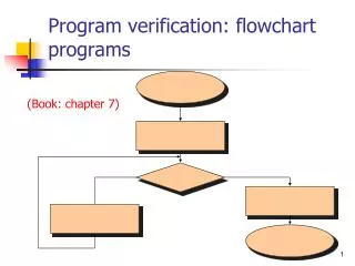
Program verification: flowchart programs (Book: chapter 7)
History • Verification of flowchart programs: Floyd, 1967 • Hoare’s logic: Hoare, 1969 • Linear Temporal Logic: Pnueli, Krueger, 1977 • Model Checking: Clarke & Emerson, 1981
Program Verification • Predicate (first order) logic. • Partial correctness, Total correctness • Flowchart programs • Invariants, annotated programs • Well founded ordering (for termination) • Hoare’s logic
Predicate (first order logic) • Variables, functions, predicates • Terms • Formulas (assertions)
Signature • Variables: v1, x, y18 Each variable represents a value of some given domain (int, real, string, …). • Function symbols: f(_,_), g2(_), h(_,_,_). Each function has an arity (number of paramenters), a domain for each parameter, and a range. f:int*int->int (e.g., addition), g:real->real (e.g., squareroot) A constant is a predicate with arity 0. • Relation symbols: R(_,_), Q(_). Each relation has an arity, and a domain for each parameter. R : real*real (e.g., greater than). Q : int (e.g., is a prime).
Terms • Terms are objects that have values. • Each variable is a term. • Applying a function with arity n to n terms results in a new term. Examples: v1, 5.0, f(v1,5.0), g2(f(v1,5.0)) More familiar notation: sqr(v1+5.0)
Formulas • Applying predicates to terms results in a formula. R(v1,5.0), Q(x) More familiar notation: v1>5.0 • One can combine formulas with the boolean operators (and, or, not, implies). R(v1,5.0)->Q(x) x>1 -> x*x>x • One can apply existentail and universal quantification to formulas. x Q(X) x1 R(x1,5.0) x y R(x,y)
A model, A proofs • A model gives a meaning (semantics) to a first order formula: • A relation for each relation symbol. • A function for each function symbol. • A value for each variable. • An important concept in first order logic is that of a proof. We assume the ability to prove that a formula holds for a given model. • Example proof rule (MP) :
Flowchart programs Input variables: X=x1,x2,…,xl Program variables: Y=y1,y2,…,ym Output variables: Z=z1,z2,…,zn start Z=h(X,Y) Y=f(X) halt
Assignments and tests T F Y=g(X,Y) t(X,Y)
Initial condition start Initial condition: the values for the input variables for which the program must work. x1>=0 /\ x2>0 (y1,y2)=(0,x1) y2>=x2 F T (y1,y2)=(y1+1,y2-x2) (z1,z2)=(y1,y2) halt
The input-output claim start The relation between the values of the input and the output variables at termination. x1=z1*x2+z2 /\ 0<=z2<x2 (y1,y2)=(0,x1) y2>=x2 T F (y1,y2)=(y1+1,y2-x2) (z1,z2)=(y1,y2) halt
Partial correctness, Termination, Total correctness • Partial correctness: if the initial condition holds and the program terminates then the input-output claim holds. • Termination: if the initial condition holds, the program terminates. • Total correctness: if the initial condition holds, the program terminates and the input-output claim holds.
start (y1,y2)=(0,x1) y2>=x2 F T (y1,y2)=(y1+1,y2-x2) (z1,z2)=(y1,y2) halt Subtle point: The program is partially correct with respect to x1>=0/\x2>=0 and totally correct with respect to x1>=0/\x2>0
Annotating a scheme start A Assign an assertion for each pair of nodes. The assertion expresses the relation between the variable when the program counter is located between these nodes. (y1,y2)=(0,x1) B T F y2>=x2 C D (y1,y2)=(y1+1,y2-x2) (z1,z2)=(y1,y2) E halt
Invariants • Invariants are assertions that hold at each state throughout the execution of the program. • One can attach an assertion to a particular location in the code:e.g., at(B) (B).This is also an invariant; in other locations, at(B) does not hold hence the implication holds. • If there is an assertion attached to each location, (A), (B), (C), (D), (E), then their disjunction is also an invariant:(A)\/(B)\/ (C)\/(D)\/(E)(since location is always at one of these locations).
Annotating a scheme with invariants start A A): x1>=0 /\ x2>=0 B): x1=y1*x2+y2 /\ y2>=0 C): x1=y1*x2+y2 /\ y2>=0 /\ y2>=x2 D):x1=y1*x2+y2 /\ y2>=0 /\ y2<x2 E):x1=z1*x2+z2 /\ 0<=z2<x2 Notice: (A) is the initial condition, Eis the input-output condition. (y1,y2)=(0,x1) B T F y2>=x2 C D (y1,y2)=(y1+1,y2-x2) (z1,z2)=(y1,y2) E A)Is theprecondition of (y1,y2)=(0,x1) and B) is its postcondition halt
Preliminary:Relativizing assertions A (B) : x1= y1 * x2 + y2 /\ y2 >= 0 Relativize B) w.r.t. the assignment, obtaining B) [Y\g(X,Y)] (I.e., (B) expressed w.r.t. variables at A.) (B)A =x1=0 * x2 + x1 /\ x1>=0 Think about two sets of variables,before={x, y, z, …} after={x’,y’,z’…}. Rewrite (B) using after, and the assignment as a relation between the set of variables. Then eliminate after by substitution. Here: x1’=y1’ * x2’ + y2’ /\ y2’>=0 /\x1’=x1 /\ x2’=x2 /\ y1’=0 /\ y2’=x1now eliminate x1’, x2’, y1’, y2’. Y=g(X,Y) (y1,y2)=(0,x1) B A (y1,y2)=(0,x1) B
Preliminary:Relativizing assertions A (B)A Y=g(X,Y) (y1,y2)=(0,x1) B A): Y=g(X,Y) A (B) (y1,y2)=(0,x1) B
Verification conditions: assignment A A) B)A whereB)A =B)[Y\g(X,Y)] A): x1>=0 /\ x2>=0 B): x1=y1*x2+y2 /\ y2>=0 B)A= x1=0*x2+x1 /\ x1>=0 Y=g(X,Y) (y1,y2)=(0,x1) B A (y1,y2)=(0,x1) B
Second assignment C): x1=y1*x2+y2 /\ y2>=0 /\ y2>=x2 B): x1=y1*x2+y2 /\ y2>=0 B)C: x1=(y1+1)*x2+y2-x2 /\ y2-x2>=0 C (y1,y2)=(y1+1,y2-x2) B
Third assignment D):x1=y1*x2+y2 /\ y2>=0 /\ y2<x2 E):x1=z1*x2+z2 /\ 0<=z2<x2 E)D: x1=y1*x2+y2 /\ 0<=y2<x2 D (z1,z2)=(y1,y2) E
Verification conditions: tests B T F B) /\ t(X,Y) C) B) /\¬t(X,Y) D) B): x1=y1*x2+y2 /\y2>=0 C): x1=y1*x2+y2 /\ y2>=0 /\ y2>=x2 D):x1=y1*x2+y2 /\ y2>=0 /\ y2<x2 t(X,Y) C D B T F y2>=x2 C D
C) B) t(X,Y) ¬t(X,Y) Verification conditions: tests B T F t(X,Y) C D B T F y2>=x2 C D
Partial correctness proof:An induction on length of execution Initially, states satisfy the initial conditions. Then, passing from one set of states to another, we preserve the invariants at the appropriate location. We prove: starting with a state satisfying the initial conditions, if are at a point in the execution, the invariant there holds. Not a proof of termination! A) no B) yes start A C) (y1,y2)=(0,x1) B T F no B) y2>=x2 C D yes (y1,y2)=(y1+1,y2-x2) (z1,z2)=(y1,y2) E D) halt
Initial condition: x>=0 Input-output claim: z=x! Exercise: prove partial correctness start (y1,y2)=(0,1) F T y1=x (y1,y2)=(y1+1,(y1+1)*y2) z=y2 halt
What have we achieved? • For each statement S that appears between points X and Y we showed that if the control is in X when (X) holds (the precondition of S) and S is executed, then (Y) (the postcondition of S) holds. • Initially, we know that (A) holds. • The above two conditions can be combined into an induction on the number of statements that were executed: • If after n steps we are at point X, then (X) holds.
(A) : x>=0 (F) : z^2<=x<(z+1)^2 z is the biggest number that is not greater than sqrt x. start A (y1,y2,y3)=(0,0,1) B y2=y2+y3 C false true y2>x D E (y1,y3)=(y1+1,y3+2) z=y1 F halt Another example
1+3+5+…+(2n+1)=(n+1)^2 y2 accumulates the above sum, until it is bigger than x. y3 ranges over odd numbers 1,3,5,… y1 is n-1. start A (y1,y2,y3)=(0,0,1) B y2=y2+y3 C false true y2>x D E (y1,y3)=(y1+1,y3+2) z=y1 F halt Some insight
It is usually sufficient to have one invariant for every loop (cycle in the program’s graph). We will have (C)=y1^2<=x /\ y2=(y1+1)^2 /\ y3=2*y1+1 start A (y1,y2,y3)=(0,0,1) B y2=y2+y3 C false true y2>x D E (y1,y3)=(y1+1,y3+2) z=y1 F halt Invariants
By backwards substitution in (C). (C)=y1^2<=x /\ y2=(y1+1)^2 /\ y3=2*y1+1 (B)=y1^2<=x /\ y2+y3=(y1+1)^2 /\ y3=2*y1+1 start A (y1,y2,y3)=(0,0,1) B y2=y2+y3 C false true y2>x D E (y1,y3)=(y1+1,y3+2) z=y1 F halt Obtaining (B)
(A)=x>=0 (B)=y1^2<=x /\ y2+y3=(y1+1)^2 /\ y3=2*y1+1 (B) relativized is 0^2<=x /\ 0+1=(0+1)^2 /\ 1=2*0+1 Simplified: x>=0 start A (y1,y2,y3)=(0,0,1) B y2=y2+y3 C false true y2>x D E (y1,y3)=(y1+1,y3+2) z=y1 F halt Check assignment condition
By backwards substitution in (B). (B)=y1^2<=x /\ y2+y3=(y1+1)^2 /\ y3=2*y1+1 (D)=(y1+1)^2<=x /\ y2+y3+2=(y1+2)^2 /\ y3+2=2*(y1+1)+1 start A (y1,y2,y3)=(0,0,1) B y2=y2+y3 C false true y2>x D E (y1,y3)=(y1+1,y3+2) z=y1 F halt Obtaining (D)
(C)=y1^2<=x /\ y2=(y1+1)^2 /\ y3=2*y1+1 (C)/\y2<=x) (D) (D)=(y1+1)^2<=x /\ y2+y3+2=(y1+2)^2 /\ y3+2=2*(y1+1)+1 start A (y1,y2,y3)=(0,0,1) B y2=y2+y3 C false true y2>x D E (y1,y3)=(y1+1,y3+2) z=y1 F halt Checking
y1^2<=x /\ y2=(y1+1)^2 /\ y3=2*y1+1 /\y2<=x (y1+1)^2<=x /\ y2+y3+2=(y1+2)^2 /\ y3+2=2*(y1+1)+1 y1^2<=x /\ y2=(y1+1)^2 /\ y3=2*y1+1 /\y2<=x (y1+1)^2<=x /\ y2+y3+2=(y1+2)^2 /\ y3+2=2*(y1+1)+1 y1^2<=x /\ y2=(y1+1)^2 /\ y3=2*y1+1 /\y2<=x (y1+1)^2<=x /\ y2+y3+2=(y1+2)^2 /\ y3+2=2*(y1+1)+1
Still needs to: Calculate (E) by substituting backwards from (F). Check that (C)/\y2>x(E) Not finished! start A (y1,y2,y3)=(0,0,1) B y2=y2+y3 C false true y2>x D E (y1,y3)=(y1+1,y3+2) z=y1 F halt
Exercise: prove partial correctness. Initially: x1>0/\x2>0. At termination: z1=gcd(x1,x2). start (y1,y2)=(x1,x2) y1=y2 F T y1>y2 F T z1=y1 y2=y2-y1 y1=y1-y2 halt
Annotation of program with invariants gcd(y1,y2)=gcd(x1,x2)/\y1>0/\y2>0/\y1>y2 start gcd(y1,y2)=gcd(x1,x2)/\y1>0/\y2>0/\y1<y2 A x1>0 /\ x2>0 (y1,y2)=(x1,x2) gcd(y1,y2)=gcd(x1,x2)/\y1>0/\y2>0 B gcd(y1,y2)=gcd(x1,x2)/\y1>0/\y2>0/\y1y2 y1=y2 T F D G y1=gcd(x1,x2) F T y1>y2 z1=y1 E F y2=y2-y1 y1=y1-y2 H z1=gcd(x1,x2) halt
Part 1 (A)=x1>0 /\ x2>0 start (B)=gcd(y1,y2)=gcd(x1,x2)/\y1>0/\y2>0 A (B)’rel= gcd(x1,x2)=gcd(x1,x2)/\x1>0/\x2>0 (y1,y2)=(x1,x2) (A) (B)’rel B y1=y2 T F D G F T y1>y2 z1=y1 E F y2=y2-y1 y1=y1-y2 H halt
Part 2a (B)= gcd(y1,y2)=gcd(x1,x2)/\y1>0/\y2>0 start (D)=gcd(y1,y2)=gcd(x1,x2)/\y1>0/\y2>0/\y1y2 A (y1,y2)=(x1,x2) (B)/\¬(y1=y2) (D) B y1=y2 T F D G F T y1>y2 z1=y1 E F y2=y2-y1 y1=y1-y2 H halt
Part 2b (B)= gcd(y1,y2)=gcd(x1,x2)/\y1>0/\y2>0 start (G)=y1=gcd(x1,x2) A (B)/\(y1=y2) (G) (y1,y2)=(x1,x2) B y1=y2 T F D G F T y1>y2 z1=y1 E F y2=y2-y1 y1=y1-y2 H halt
Part 3 (F)=(gcd(y1,y2)=gcd(x1,x2)/\y1>0/\y2>0/\y1>y2 start (D)/\(y1>y2) (F) (E)=gcd(y1,y2)=gcd(x1,x2)/\y1>0/\y2>0/\y1<y2 A (D)/\¬(y1>y2) (E) (y1,y2)=(x1,x2) B (D)= gcd(y1,y2)=gcd(x1,x2)/\y1>0/\y2>0/\y1y2 F T y1=y2 G D F T y1>y2 z1=y1 E F y2=y2-y1 y1=y1-y2 H halt
(B)’relE=gcd(y1,y2-y1)=gcd(x1,x2)/\y1>0/\y2-y1>0 Part 4 (F)= gcd(y1,y2)=gcd(x1,x2)/\y1>0/\y2>0/\y1>y2 (B)’relF=gcd(y1-y2,y2)=gcd(x1,x2)/\y1-y2>0/\y2>0 start (E)= gcd(y1,y2)=gcd(x1,x2)/\y1>0/\y2>0/\y1<y2 A x1>0 /\ x2>0 (y1,y2)=(x1,x2) (B)= gcd(y1,y2)=gcd(x1,x2)/\y1>0/\y2>0 B y1=y2 T F D G F T y1>y2 z1=y1 E F y2=y2-y1 y1=y1-y2 H halt (E) (B)’rel1 (F) (B)’rel2
Annotation of program with invariants start (H)’rel= y1=gcd(x1,x2) A (y1,y2)=(x1,x2) B (G)= y1=gcd(x1,x2) y1=y2 T F D G F T y1>y2 z1=y1 E F (H)= z1=gcd(x1,x2) y2=y2-y1 y1=y1-y2 H halt (G) (H)’rel2
Well-founded sets • Partially ordered set (W,<): • If a<b and b<c then a<c (transitivity). • If a<b then not b<a (asymmetry). • Nota<a (irreflexivity). • Well-founded set (W,<): • Partially ordered. • No infinite decreasing chain a1>a2>a3>…
Examples for well founded sets • Natural numbers with the bigger than relation. • Finite sets with the set inclusion relation. • Strings with the substring relation. • Tuples with alphabetic order: • (a1,b1)>(a2,b2) iff a1>a2 or [a1=a2 and b1>b2]. • (a1,b1,c1)>(a2,b2,c2) iff a1>a2 or [a1=a2 and b1>b2] or [a1=a2 and b1=b2 and c1>c2].
y2 starts as x1. Each time the loop is executed, y2 is decremented. y2 is natural number The loop cannot be entered again when y2<x2. true y2>=x2 C Why does the program terminate start A (y1,y2)=(0,x1) B false D (y1,y2)=(y1+1,y2-x2) (z1,z2)=(y1,y2) E halt
Proving termination • Choose a well-founded set (W,<). • Attach a function u(N) to each point N. • Annotate the flowchart with invariants, and prove their consistency conditions. • Prove that j(N) (u(N) in W).
Show that u(M)>=u(N)’rel. At least once in each loop, show that u(M)>u(N). How not to stay in a loop? M S N M T N