Download
1 / 19
190 likes | 375 Vues
Metr 51: Scientific Computing II Lecture 9 : Lidar Plotting Techniques. Allison Charland 3 April 2012. Reminder. Two weeks of Matlab left! Matlab Final will be on April 19 th Then on to HTML and creating a personal webpage. Doppler Lidar Theory. Movement of aerosols by wind.

E N D
Metr 51: Scientific Computing IILecture 9: Lidar Plotting Techniques Allison Charland 3 April 2012
Reminder • Two weeks of Matlab left! • Matlab Final will be on April 19th • Then on to HTML and creating a personal webpage
Doppler Lidar Theory Movement of aerosols by wind Infrared light reflected from aerosols Emitted infrared light The shift in frequency of the return echo is related to the movement of aerosols. The faster the aerosols move, the larger the shift in frequency. From this, the wind speed relative to the light beam can be measured.
Doppler wind lidar • Halo Photonics, Ltd. Stream Line 75 • 1.5 micron • Eye-safe • 75 mm aperture all-sky optical scanner • Min Range: 80 m • Max Range: 10km • 550 user defined range gates (24 m) • Temporal resolution: 0.1-30 s • Measurements: • Backscatter Intensity • Doppler Radial Velocity
Lidar Scanning Techniques 30o 70o 95o • Multiple elevation and azimuth angles can be adjusted to create different types of scans. • DBS (Doppler Beam Swinging): • Wind Profile • Stare: Vertically pointing beam • RHI (Range Height Indicator): • Fixed azimuth angle with varying elevation angles • PPI (Plan Position Indicator): • Fixed elevation angle with varying azimuth angles
DBS Data Date & Time(UTC) Height (m AGL) Wind Direction & Wind Speed (ms-1) • Remove 225 heading • Use load to read in the data then create wind speed and direction profiles. • What if you have multiple files that you want to plot using one code?
Plotting multiple profiles • You have three files that you want to plot: wind_profile_0900PST.txt, wind_profile_1200PST.txt, and wind_profile_1500PST.txt • Create a character string array called filenames filenames = [‘wind_profile_0900PST.txt’;… ‘wind_profile_1200PST.txt’;‘wind_profile_1500PST.txt’]; Hint: filenames must all be the same character length • Create a variable for the number of files you have Num = 3;
Plotting multiple profiles • Now you want to create a for loop that will go from 1 to the number of files you have and load and plot each file. • Each time you loop through you want to reset the filename that is being read. • Set your values of height, wind direction and wind speed. • Plot your variables. • Clear variables so that the next time through the loop they will be replaced.
Plotting multiple profiles for i =1:Num f = filenames(i,:); load f; data = f; clear f; height = data(:,1); wind_dir = data(:,2); wind_speed = data(:,3); figure(1);clf; plot(wind_dir, height, ‘+k’); hold on; plot(wind_speed, height, ‘k’); hold on; clear data; clear height; clear wind_dir; clear wind_speed; end %for
Plotting multiple profiles • To plot each profile as a separate figure replace figure(1);clf; with figure(i);clf; • To save each figure as a jpeg, use saveasafter your figure is complete figure_name = [‘profile_’i’.jpg’]; saveas(gcf,figure_name); • Each time through the loop the figure_name will be reset and saved with the new number i.
Stare Lidar Data Date & Time(UTC) There is one data file per hour
Stare Data • The load command cannot be used for stare data because the number of columns changes throughout the data file from 3 to 4 after each scan. • Fastest way to plot stare data is using xlsread • This reads in an excel spreadsheet then later using loops the data can be separated into specific variables. • The first step is to load the stare data file into excel space delimited then save it as an excel file with the extension .xlsx (for Microsoft 2010).
Stare Data • Before loading the data, set up the height array. • Heights will always be the same throughout a stare file. • height = 0:225; • height = (height + 0.5)*24; • height = height';
Stare Data • Read in the datafile • data = xlsread(filename.xlsx); • j = hour; %The hour of the particular data file • fprintf('Completed %2.0f \n', j) • Set conditions for start of data columns • c1=2; • if j > 1 • k=17; • p=18; • elseif j==1 • k=9; • p=10; • end • if j >= 4 • c1=1; • end %if • if j >= 18 • c1=2; • end %if
Splitting the data count = 0; n = 2100; for i=1:n count = count +1; time(count) = data(k,c1); k=k+226; V = data(p:p+100,3)'; V_2 = data(p+100:p+224,2)'; V_new(count,:) = [V V_2]; B = data(p:p+100,4)'; B_2 = data(p+100:p+224,3)'; B_new(count,:) = [B B_2]; p=p+226; end %for fprintf('Completed split \n')
Stare Data • Change time from UTC to PST • Depends on Daylight Savings • for w = 1:length(time) • if time(w) < 7; • time(w) = 24 - (7-time(w)); • else • time(w) = time(w)-7; • end %if • end %for
Transpose the data Transpose the data B_new = B_new'; V_new = V_new'; time =time' ;
Plotting Stare Data figure(1);clf; pcolor(time,height,V_new);hold on; shading interp; ylim([0 2400]) xlabel('Time (PST) '); ylabel('Height (m AGL)'); title('Vertical Velocity (m s^-^1)') caxis([-5 4]) colorbar Show Example
Stare Data • The example shown is the raw data. • A filter algorithm can be used to eliminate invalid data including near the surface and aloft where the signal is no longer retrieved. • The algorithm code will be available on D2L. • Multiple files could be read in and plotting using the same technique as earlier to plot multiple wind profiles. • The problem is that the figures created will have so much detail that there may be issues copying them.