Download
1 / 32
320 likes | 479 Vues
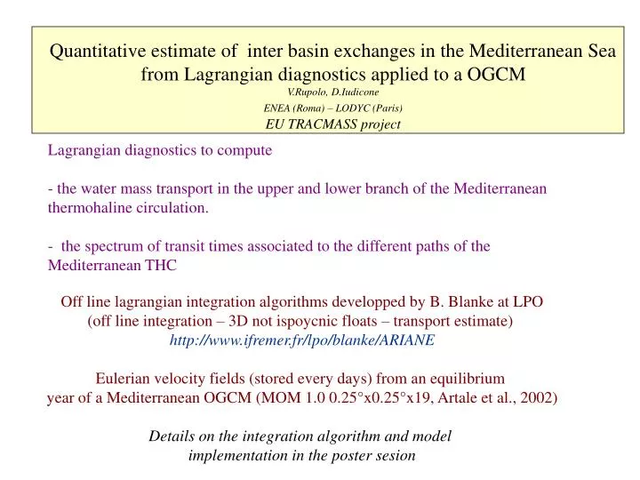
Quantitative estimate of inter basin exchanges in the Mediterranean Sea from Lagrangian diagnostics applied to a OGCM V.Rupolo, D.Iudicone ENEA (Roma) – LODYC (Paris) EU TRACMASS project. Lagrangian diagnostics to compute

E N D
Quantitative estimate of inter basin exchanges in the Mediterranean Sea from Lagrangian diagnostics applied to a OGCM V.Rupolo, D.Iudicone ENEA (Roma) – LODYC (Paris) EU TRACMASS project Lagrangian diagnostics to compute - the water mass transport in the upper and lower branch of the Mediterranean thermohaline circulation. - the spectrum of transit times associated to the different paths of the Mediterranean THC Off line lagrangian integration algorithms developped by B. Blanke at LPO (off line integration – 3D not ispoycnic floats – transport estimate) http://www.ifremer.fr/lpo/blanke/ARIANE Eulerian velocity fields (stored every days) from an equilibrium year of a Mediterranean OGCM (MOM 1.0 0.25°x0.25°x19, Artale et al., 2002) Details on the integration algorithm and model implementation in the poster sesion
The Mediterranean is an evaporative basin and the Gibraltar strait is a source of intermediate water ? ※ In the 90’ have been observed dramatic changes in the deep water formation and in the vertical stratification in the EM. How/when they reflect in the Gibraltar Output ?
Qualitative visualisation of the upper branch of the THC About 60 000 particles uniformly released in the surface layers. colours indicate depth from surface (blu) to 1000 m. (yellow)
Qualitative visualisation of the lower branch of the THC in the East Mediterranean About 60 000 particles uniformly released in the surface layers. colours indicate depth from 200 m (blu) to 1700 m. (yellow)
Qualitative visualisation of the lower branch of the THC in the West Mediterranean About 60 000 particles uniformly released in the surface layers. colours indicate depth from 50 m (blu) to 1700 m. (yellow)
The global TH cell appears to be composed by several different paths - Quantitative estimate by releasing about 500 000 particles in the inflow in the Alborean Sea and integrating them till they cross again the same section. - For each particle hydrological characteristics and transit time are stored when crossing one of the ‘transparent’ sections in the basin. Sub division in different paths by checking the arrival times in the transparent sections
Total TH cell = Global cell + Western Cell + Fast recirculation Distribution of arrival times
Global Cell, Upper Branch Red arrows indicate the lower branch
Global Cell, Lower Branch Water Mass transformation SIC SARD NW ALB LEV SIC ADR oo Mean values T and S of the outflowing water in the Alborean Sea strongly depend on mixing between water of eastern origin with fresher and cooler water in the North Western Mediterranean paths P2 and P3 (strongly depending on deep convection in the NWM)
Global Cell, Lower Branch Arrival times
Characteristic times Experimental arrival times distribution P(t) Tmode : P(Tmode) > P(t) t Tfirst=first arrival time Cumulative F(t) = 0t P(t’)dt’/ 0 P(t’)dt’ median tm: F(tm) = 0.5 Percentage of water connecting the two sections in a time smaller than t Concentration in the basin C(t)=1-F(t) Tres 0 C(t’)dt’ Typical times Ti if in some ranges C(t) e –t/Ti
Often to fit the experimental distribution of the arrival times is used - without dynamical arguments for its revelance – the solution of the one-dimensional advective-diffusive equation G(t*, , ) = ·(4 2t*3) –1/2 exp{- 2(t*-1) 2 /4 2 t*}, where is the mean arrival time and is a measure of the width of the curve (dispersal) , same Great , diffusive behaviour (long tails) Great , advective behaviour (peaked around )
Global cell, total lower branch Transit times distribution from Sicily to Alborean Sea - - total P1 P2 P3
Global cell, P1 lower branch Transit times distribution from Sicily to Alborean Sea
Global cell, P2 lower branch Transit times distribution from Sicily to Alborean Sea
Global cell, P3 lower branch Transit times distribution from Sicily to Alborean Sea
Water Mass composition and Age ’Classical’ quantitative Water Mass Analysis: thetracer concentration is expressed as a linear combination of N source-water values: = a1 1 + a2 2 + ………….. ….. +aN N ai >0, ai=1 The coefficient ai can be expressed (Haine and Hall, 2002) as: ai = Ci 0d Gi’(r, | 1), ai >0, ai=1 where Gi’ = distribution of transit times from the source region i to r Lagrangian approach The water-mass component is definedby the geographical path from two given initial and final sections where particles are released and stopped and the related distribution of the arrival times P() can be subdivided in N distribution P i () corresponding to N different paths connecting the two sections: P()= i P i() In equilibrium the arrival time distributions corresponds to the age spectrum of the considered transport between the two sections, then it is possible to compute the relative composition of a water parcel in the final section in terms as a function of the water ‘age’ (elapsed time from the initial to the final section).
Global cell, total lower branch Cumulative functions - - total P1 P2 P3 Fi/Ftot: Relative Composition As a function of the age
Summary • Lagrangian diagnostics powerful tool to fully exploit results • from Eulerian OGCM (detailed description of circulation paths) • - Analysis of the transit times distributions particularly • interesting (transmission of an anomalous signal, accident, • pollution)
Water Mass composition Quantitative Water Mass Analysis Composition of a water parcel in terms of the different fractions of source waters. Tracer concentration as a linear combination of N source-water value: T= a1T1 + a2T2 + ….. +aNTN S= a1S1 + a2S2 + ….. +aNSN ai >0, ai=1 A water-mass component is defined by the geographical location of the formation site, or (Lagrangian approach) by the geographical path from two given initial and final sections
Tracer Green’s Function t(r,t) + [(r,t)]= S(r,t) • is a linear opeartor including advection and diffusive mixing S is a tracer source or sink The Green’s function G(r,t|r’,t’) is the solution to the related problem tG(r,t) + [G(r,t)]= (r-r’)(t-t’) G is the response of tracer concentration to an instantaneous impulse at time t’ and position r’ in the interior. Considered as a function of r, t, r’ and t. G captures complete information about transport processes in the flow. The tracer field from a continuous source is a superposition of individual pulses. (r,t) =d3r’dt’ S(r’,t) G(r,t|r’,t’) S(r’,t’)G(r,t|r’,t’)/ (r,t)is the fraction of tracer at r that released at r’ has resided In the ocean a time =t-t’ and is a distribution of transit timefrom r to r’.
Tracer Boundary propagator tG’(r,t) + [G’(r,t)]= 0 The concentration boundary condition are G’=(r-r’,t-t’), where r’ is on the boundary surface . The interior tracer concentration can be built from G’: (r,t) = d2r’ tot dt’ (r,t’) G’(r,t|r’,t’) Where (r,t) (r) is a known time variation of the concentration on The interior field is obtained by multiplying G’ with the boundary concentration and integrating. From all the possible pathways from to (r,t), G’(r,t|r’,t’)dt’d2r’ is the fraction that originated from the boundary region d2r’ in the time interval (t’,t’+dt’). G’(r,t|r’,t’) is a joint distribution function describing the water-mass composition at r and t from different surface-source regions and different times. Considering a surface concentration steady in time and piece-wise constant over a series of N surface patches 1 … N we then have: (r) = (1)1 0d G1’(r, | 1) + … + (N)N 0d GN’(r, | N) =t-t0
P()= experimental arrival time distribution that can be decomposed in N arrival time distribution Pi() : i Pi() = P() corresponding to N different path connecting initial and final section F(t) = 0td P() (t)= F(t)/F() represents the percentage of water , with regard to the total flow, connecting the initial and final section in a time smaller than t Fi(t) = 0td Pi() i(t) = Fi(t)/F(t) = 0td Pi() [ 0td P()] –1,i i() = 1 i represents the percentage of water, with regard to the flow younger than t, that connects the initial and final section following the i-th path.
Arrival times distribution Total cell Global cell Western cell WC, circulating In the Tyrrhenian Fast recirculation
In one dimension, the tracer continuity equation is t + u· x-k· xx= 0, where u is the velocity, k is the diffusivity nd the only tracer source is ta x = 0. The transit time distribution function G(x,t) is the response to a boundary condition (t) at x = 0. For constant uniform u and k: G(x,t) = x · (4kt3) –1/2 exp{-(ut-x)2/4kt} An alternative form is(t*= /t) G(t*, , ) = ·(4 2t*3) –1/2 exp{- 2(t*-1) 2 /4 2 t*} This distribution depends on the mean transit time and width , that are simply Related to u and k (=x/u , =(kx)1/2/u3/2 ). This solution – without dynamical arguments for the revelance of one-dimensional Transport - is a convenient form to fit experimental arrival time distribution making freely vary the parameters (mean age) and (width)
Upwelling through the nutricline: particles are released (homogeneously) at 160 m. of depth and they are integrated till they reach the depth of 30, 15 and 5 m. standard year 1993:Fully developped EMT From 160 to 5: 0.01 Sv From 160 to 5: 0.02 Sv From 160 to 15: 0.02 Sv From 160 to 15: 0.04 Sv From 160 to 300: 0.03 Sv From 160 to 300: 0.07 Sv
Time behavior of flux through the ‘nutricline’ Red = flux at the starting section, black= flux at the ending section standard year 1993 From 160 to 5: From 160 to 5: From 160 to 15: From 160 to 15: From 160 to 30: From 160 to 30:
Summary • Relaxing model SST to satellite SST from 1988 to 1993, the general • mechanism of the EMT is reproduced • Lagrangian diagnostics make easier the analysis of the development • of the EMT as it is represented by the model and allows quantitative • estimates, in particular: • In a preconditioning phase IW inflow in the Adriatic (Aegean) decreases (increases). Probably wind induced (Samuel et al, Demirov and Pinardi) • The EMT fully develops during 1992 and 1993, the overflow from the Aegean is concentrated during two events (O(months)). The total flow over the Cretan Arcs is 1.2 1014 m3(roughly the half of he estimate of Roether et al.; 1996) • Relaxation toward pre-EMT situatiuon (qualitative behavior and estimate of characteristic time) • Moreover: Quantitative estimates of vertical transport before and after the EMT (up lifted water), Time statistics • http://clima.casaccia.enea.it/staff/rupolo