Download
1 / 21
530 likes | 1.49k Vues
PBG 650 Advanced Plant Breeding. Module 8: Estimating Genetic Variances Nested design GCA, SCA Diallel. Nested design. Also called North Carolina Design 1 Hierarchical design Two types of families Half sibs (male groups) Full-sibs (females/males). Females. Males. 1 2 3 4. 1. 5

E N D
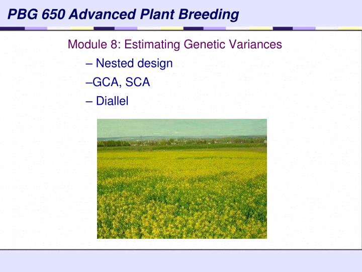
PBG 650 Advanced Plant Breeding Module 8: Estimating Genetic Variances Nested design GCA, SCA Diallel
Nested design • Also called • North Carolina Design 1 • Hierarchical design • Two types of families • Half sibs (male groups) • Full-sibs (females/males) Females Males 1 2 3 4 1 5 6 7 8 2 . . . m . . f
Nested design – one location • Might also have sets and multiple environments Linear Model Yijk= + Bi + Mj + Fk(j) + eijk See Bernardo, pg 164, for ANOVA with sets and environments
(if the parents are not inbred) Variance components from the nested design (if the parents are not inbred)
Expected Mean Squares in SAS • Random statement generates expected mean squares • Test option obtains appropriate F tests for the model specified • In the example below, cultivars are fixed, all other effects are random ProcGLM; Class Loc Rep Cultivar; Model Yield=Loc Rep(Loc) Cultivar Loc*Cultivar; Random Loc Rep(Loc) Loc*Cultivar/Test; Run; controversial (could be dropped) Source Type III Expected Mean Square Loc Var(Error) + 3 Var(Loc*Cultivar) + 7 Var(Rep(Loc)) + 21 Var(Loc) Rep(Loc) Var(Error) + 7 Var(Rep(Loc)) Cultivar Var(Error) + 3 Var(Loc*Cultivar) + Q(Cultivar) Loc*Cultivar Var(Error) + 3 Var(Loc*Cultivar) fixed effect • Proc Mixed may give better estimates of variance components
Combining Ability • General combining ability(GCA)– the average of all F1 crosses from a line (or genotype), expressed as a deviation from the population mean • The expected value of a cross is the sum of the combining ability of its two parents • Specific combining ability(SCA)– the deviation of a cross from its expected value Where X is the performance of the cross
Estimation of combining ability GCA • polycross method - allow all lines to intermate naturally • top crossing - a line is crossed to a random sample of plants from a reference population GCA and SCA • Factorial design (NC Design II) – a group of ‘male’ parents is crossed to a group of ‘female’ parents • requires mxf crosses (e.g. 5x5=25) • can be applied to two heterotic populations • Diallel – all possible crosses among a set of parents • n(n-1)/2 possible crosses without parents or reciprocals (e.g. 10x9/2=45)
Variations on the Diallel • Type of cross-classified design • With or without the parents • With or without reciprocal crosses • bulk seed from both parents if maternal effects are not important • Genotypes may be random or fixed • For random model, need many parents to adequately sample the population • Large number of crosses! • Can be divided into sets • Partial diallels can be conducted • If parents are inbred, can make paired row crosses to obtain more seed Hallauer, Carena, and Miranda (2010) pg 119-138
Griffing’s Methods (Diallels) • Method 1 • all possible crosses, including selfs • Method 2 • no reciprocals • Method 3 • no parents • Method 4 • no parents or reciprocals • most common, because parents often inbred and less vigorous For each Method, genotypes may be Model I = Fixed Model II = Random
Diallel crossing ….. …..
Random model • Usually does not include parents and reciprocals • Can be divided into sets Griffing (1956) is classic reference
Genetic variances from random model General form for variance of a variance component k=coefficient of MS fg=df of the mean square
Fixed model • GCA effects • SCA effects Lattice designs are useful Advantage: first order effects (means) are estimated with greater precision than variances
Diallel analysis with parents Gardner-Eberhart Analysis II • Gardner-Eberhart partitioning of Sums of Squares is non-orthogonal • Fit model sequentially
Factorial Mating Design Diallel Factorial (Design II)
General formula for covariance of relatives A B C D X Y r = 2XY = ACBD + ADBC Extended to include epistasis:
Epistatic Variance • Often assumed to be absent, but could bias estimates of A2 andD2 upwards • Estimation requires more complex mating designs • Expected to be smaller than A2 andD2, so larger experiments are needed for adequate precision • Coefficients are correlated with those for A2 andD2, which leads tomulticollinearity problems • For most crops, experimental estimates of epistatic variance have been small
Example of mating design to estimate epistatic variance • Design I experiment from ‘Jarvis’ and ‘Indian Chief’ maize populations • Obtained random inbred lines from each population, which were used as parents in a Design II experiment • A comparison of these values can be made to estimate epistatic variances Eberhart et al., 1966
Precision of variance components • Minimum of 50-100 progeny to adequately sample population (Bernardo’s advice, some would say more!) • Large numbers of progeny do not guarantee precise estimates of variance • Confidence intervals can be determined for estimates of variance (sets lower and upper bounds) • It’s possible in practice to obtain negative estimates of variance components, but they are theoretically impossible • large error variance • true estimate of genetic variance is close to zero • Report as zero? (may lead to bias when results are compiled across many experiments) See Bernardo, pg 166, for further details on confidence intervals
Resampling methods • Confidence interval calculations assume that the underlying distribution is normal. Work best for balanced data. • Resampling methods are useful when • underlying distributions are unknown or are not normal • we don’t know how to estimate the confidence interval • Examples • Bootstrap – resampling with replacement • Jackknife – systematically delete data points • Permutation test – data scrambling • only works when there are two or more types of families