Download
1 / 21
210 likes | 342 Vues
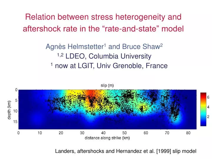
Agnès Helmstetter 1 and Bruce Shaw 2 1,2 LDEO, Columbia University 1 now at LGIT, Univ Grenoble, France. Relation between stress heterogeneity and aftershock rate in the “rate-and-state” model. Landers, aftershocks and Hernandez et al. [1999] slip model. -- Omori law R ~1/t. c.

E N D
Agnès Helmstetter1 and Bruce Shaw2 1,2 LDEO, Columbia University 1 now at LGIT, Univ Grenoble, France Relation between stress heterogeneity and aftershock rate in the “rate-and-state” model Landers, aftershocks and Hernandez et al. [1999] slip model
-- Omori law R~1/t c “Rate-and-state” model of seismicity [Dieterich 1994] Seismicity rate R(t) after a unif stress step (t) [Dieterich, 1994] • ∞ population of faults with R&S friction law • constant tectonic loading ’r Aftershock duration ta • A≈ 0.01 (friction exp.) • n≈100 MPa (P at 5km) «min» time delay c()
Coseismsic slip, stress change, and aftershocks: Planar fault, uniform stress drop, and R&S model slip shear stressseismicity rate Real data: most aftershocks occur on or close to the rupture area Slip and stress must be heterogeneous to produce an increase of and thus R on parts of the fault
Seismicity rate and stress heterogeneity Seismicity rate triggered by a heterogeneous stress change on the fault • R(t,t) : R&S model, unif stress change [Dieterich 1994] • P(t) : stress distribution (due to slip heterogeneity or fault roughness) • instantaneous stress change; no dynamic t or postseismic relaxation Goals • seismicity rate R(t) produced by a realistic P(t) • inversion of P(t) from R(t) • see also Dieterich 2005; and Marsan 2005
0 0 Slip and shear stress heterogeneity, aftershocks aftershock map synthetic R&S catalog shear stress stress drop 0 =3 MPa slip Modified «k2» slip model: u(k)~1/(k+1/L)2.3 [Herrero & Bernard, 94] stress distrtibution P()≈Gaussian
∫ R(t,)P()d -- Omori law R(t)~1/tp with p=0.93 ta Rr Stress heterogeneity and aftershock decay with time Aftershock rate on the fault with R&S model for modified k2 slip model Short timest‹‹ta : apparent Omori law with p≤1 Long timest≈ta : stress shadow R(t)<Rr
Stress heterogeneity and aftershock decay with time • Early time rate controlled by large positive • Huge increase of EQ rate after the mainshock even where u>0 and where <0 on average • Long time shadow for t≈tadue to negative • Integrating over time: decrease of EQ rate ∆N = ∫0∞[R(t) - Rr] dt ~ -0 Rrta/An • But long-time shadow difficult to detect
d L Modified k2 slip model, off-fault stress change • distance d<L from the fault: (k,d) ~ (k,0) e-kd for d«L • fast attenuation of high frequency perturbations with distance coseismic shear stress change (MPa)
stress (MPa) standard deviation d/L=0.1 d/L average stress change Modified k2 slip model, off-fault aftershocks • stress change and seismicity rate as a function of d/L • quiescence for d >0.1L
log P() 0 Stress heterogeneity and Omori law • For an exponential pdf P()~e-/owith >0 • R&S gives Omori law R(t)~1/tpwith p=1- An/o • black: global EQ rate, heterogeneous : R(t) = ∫ R(t,)P()d with o/An=5 • colored lines: EQ rate for a unif : R(t,)P() from=0 to=50 MPa p=0.8 p=1
Stress heterogeneity and Omori law • smooth stress change, or large An Omori exponent p<1 • very heterogeneous stress field, or small An • Omori p≈1 • p>1 can’t be explained by a stress step (r) postseismic relaxation (t)?
Inversion of stress distribution from aftershock rate Deviations from Omori law with p=1 due to: • (r) : spatial heterogeneity of stress step [Dieterich, 1994; 2005] • (t) : stress changes with time [Dieterich, 1994; 2000] We invert for P() from R(t) assuming (r) • solve R(t) = ∫R(t,)P()d for P() does not work for realistic catalogs (time interval too short) • fit of R(t) by∫R(t,)P()d assuming a Gaussian P() - invert for ta and * (standard deviation) - stress drop fixed (not constrained if tmax<ta) - good results on synthetic R&S catalogs
Synthetic R&S catalog:- input P() N=230 - inverted P(): fixed An ,Rr and ta An=1 MPa - Gaussian P(): - fixed An and Rr 0 = 3 MPa - invert for ta, 0 and * *=20 MPa - Gaussian P(): - fixed An , 0 and Rr - invert for ta and * Inversion of stress pdf from aftershock rate p=0.93
data, aftershocks data, `foreshocks’ fit R&S model Gaussian P() fit Omori law p=0.88 ta foreshock Rr Parkfield 2004 M=6 aftershock sequence • Fixed: An = 1 MPa 0 = 3 MPa • Inverted: *= 11 MPa ta = 10 yrs
Data, aftershocks Fit R&S model Gaussian P() Fit Omori law p=1.08 foreshocks ta Rr Landers, 1992, M=7.3, aftershock sequence • Fixed: An = 1 MPa 0 = 3 Mpa • Inverted: *= 2350 MPa ta = 52 yrs • Loading rate d/dt = An / ta = 0.02 MPa/yr • « Recurrence time » tr= ta 0/An = 156 yrs
Superstition Hills 1987 M=6.6 (South of Salton Sea 33oN) • Fixed: An = 1 MPa 0 = 3 MPa Data, aftershocks Fit R&S model Gaussian P() Fit Omori law p=1.3 Elmore Ranch M=6.2 Rr foreshocks
data, aftershocks Fit R&S model Gaussian P() Fit Omori law p=0.68 foreshocks ta Rr Morgan Hill, 1984 M=6.2, aftershock sequence • Fixed: An = 1 MPa 0 = 3 Mpa • Inverted: *= 6.2 MPa ta = 26 yrs • Loading rate d/dt = An / ta = 0.04 MPa/yr • «Recurrence time» tr= ta 0/An = 78 yrs
Data, aftershocks Fit R&S model Gaussian P() Fit Omori law p=0.89 foreshocks ta Rr Stacked aftershock sequences, Japan (80, 3<M<5, z<30) • Fixed: An = 1 MPa 0 = 3 Mpa • Inverted: *= 12 MPa ta = 1.1 yrs • Loading rate d/dt = An / ta = 0.9 MPa/yr • «Recurrence time» tr= ta 0/An = 3.4 yrs [Peng et al., in prep, 2006]
Inversion of P() from R(t) for real aftershock sequences Sequence p * (MPa)ta (yrs) Morgan Hill M=6.2, 1984 0.68 6.2 78. Parkfield M=6.0, 2004 0.88 11. 10. Stack, 3<M<5, Japan* 0.89 12. 1.1 San Simeon M=6.5 2003 0.93 18. 348. Landers M=7.3, 1992 1.08 ** 52. Northridge M=6.7, 1994 1.09 ** 94. Hector Mine M=7.1, 1999 1.16 ** 80. Superstition-Hills, M=6.6,1987 1.30 ** ** ** : we can’t estimate * because p>1 (inversion gives *=inf) * [Peng et al., in prep 2005]
Conclusion R&S model with stress heterogeneity gives: - “apparent” Omori law with p≤1 for t<ta, if * ›0 , p1 with «heterogeneity» * • quiescence: • for t≈ta on the fault, • or for r/L>0.1 off of the fault - in space : clustering on/close to the rupture area
Problems / future work Inversion of stress drop not constrained if catalog too short trade-off between ta and 0 trade-off between space and time stress variations can’t explain p>1 : post-seismic stress relaxation? or other model? An? - 0.002 or 1MPa?? - heterogeneity of An could also produce change in p value secondary aftershocks? renormalize Rr but does not change p ? [Ziv & Rubin 2003] submited to JGR 2005, see draft at www.ldeo.columbia.edu/~agnes