Download
1 / 1
10 likes | 156 Vues
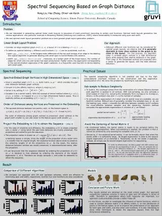
Spectral Sequencing Based on Graph Distance. Rong Liu, Hao Zhang, Oliver van Kaick {lrong, haoz, ovankaic} @ cs.sfu.ca. School of Computing Science, Simon Fraser University, Burnaby, Canada. Introduction. Problem.

E N D
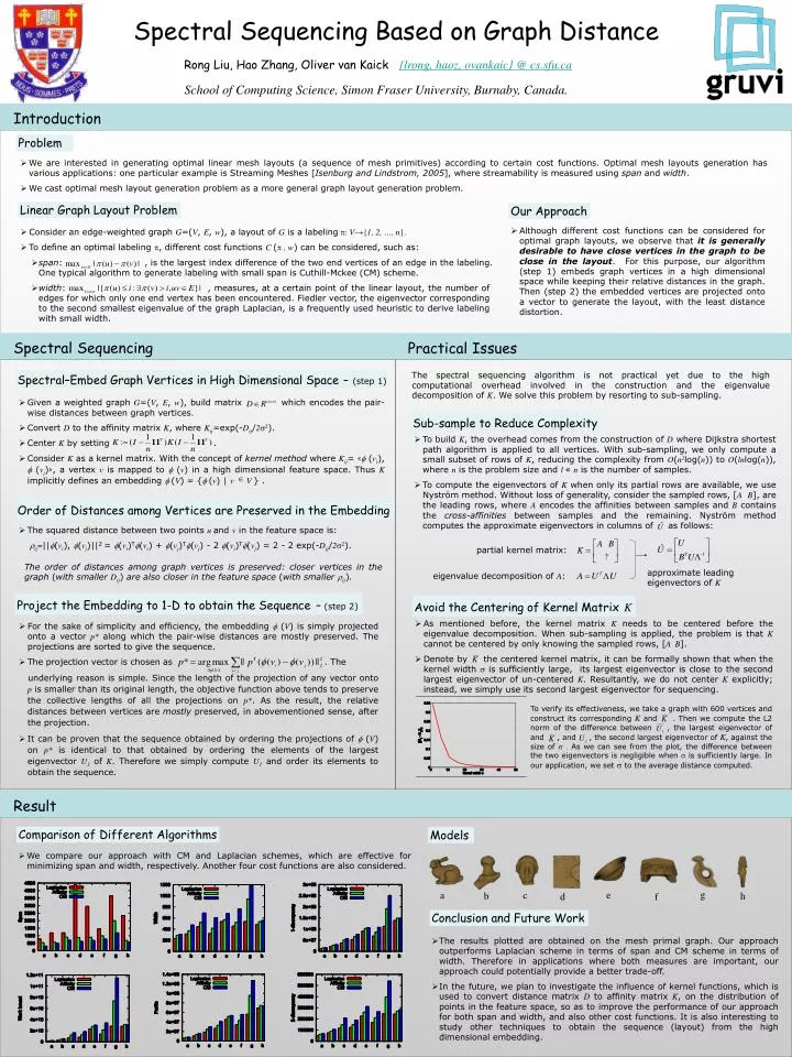
Spectral Sequencing Based on Graph Distance Rong Liu, Hao Zhang, Oliver van Kaick {lrong, haoz, ovankaic} @ cs.sfu.ca School of Computing Science, Simon Fraser University, Burnaby, Canada. Introduction Problem • We are interested in generating optimal linear mesh layouts (a sequence of mesh primitives) according to certain cost functions. Optimal mesh layouts generation has various applications: one particular example is Streaming Meshes [Isenburg and Lindstrom, 2005], where streamability is measured using span and width. • We cast optimal mesh layout generation problem as a more general graph layout generation problem. Linear Graph Layout Problem Our Approach • Although different cost functions can be considered for optimal graph layouts, we observe that it is generally desirable to have close vertices in the graph to be close in the layout. For this purpose, our algorithm (step 1) embeds graph vertices in a high dimensional space while keeping their relative distances in the graph. Then (step 2) the embedded vertices are projected onto a vector to generate the layout, with the least distance distortion. • Consider an edge-weighted graph G=(V, E, w), a layout of G is a labelingp: V→{1, 2, …, n}. • To define an optimal labeling p, different cost functions C (p , w) can be considered, such as: • span: , is the largest index difference of the two end vertices of an edge in the labeling. One typical algorithm to generate labeling with small span is Cuthill-Mckee (CM) scheme. • width: , measures, at a certain point of the linear layout, the number of edges for which only one end vertex has been encountered. Fiedler vector, the eigenvector corresponding to the second smallest eigenvalue of the graph Laplacian, is a frequently used heuristic to derive labeling with small width. Spectral Sequencing Practical Issues The spectral sequencing algorithm is not practical yet due to the high computational overhead involved in the construction and the eigenvalue decomposition of K. We solve this problem by resorting to sub-sampling. Spectral–Embed Graph Vertices in High Dimensional Space - (step 1) • Given a weighted graph G=(V, E, w), build matrix which encodes the pair-wise distances between graph vertices. • Convert D to the affinity matrix K, where Kij=exp(-Dij/2s2). • Center K by setting . • Consider K as a kernel matrix. With the concept of kernel method where Kij= ‹f (vi), f (vj)›, a vertex v is mapped to f (v) in a high dimensional feature space. Thus K implicitly defines an embedding f (V) = {f (v) | v V } . Sub-sample to Reduce Complexity • To build K, the overhead comes from the construction of D where Dijkstra shortest path algorithm is applied to all vertices. With sub-sampling, we only compute a small subset of rows of K, reducing the complexity from O(n2log(n)) to O(lnlog(n)), where n is the problem size and l « n is the number of samples. • To compute the eigenvectors of K when only its partial rows are available, we use Nyström method. Without loss of generality, consider the sampled rows, [A B], are the leading rows, where A encodes the affinities between samples and B contains the cross-affinities between samples and the remaining. Nyström method computes the approximate eigenvectors in columns of as follows: Order of Distances among Vertices are Preserved in the Embedding • The squared distance between two points u and v in the feature space is: • rij=||f(vi), f(vj)||2 = f(vi)Tf(vi) + f(vj)Tf(vj) - 2 f(vi)Tf(vj) = 2 - 2 exp(-Dij/2s2). partial kernel matrix: The order of distances among graph vertices is preserved: closer vertices in the graph (with smaller Dij) are also closer in the feature space (with smaller rij). approximate leading eigenvectors of K eigenvalue decomposition of A: Project the Embedding to 1-D to obtain the Sequence- (step 2) Avoid the Centering of Kernel MatrixK • As mentioned before, the kernel matrix K needs to be centered before the eigenvalue decomposition. When sub-sampling is applied, the problem is that K cannot be centered by only knowing the sampled rows, [A B]. • Denote by the centered kernel matrix, it can be formally shown that when the kernel width s is sufficiently large, its largest eigenvector is close to the second largest eigenvector of un-centered K. Resultantly, we do not center K explicitly; instead, we simply use its second largest eigenvector for sequencing. • For the sake of simplicity and efficiency, the embedding f (V) is simply projected onto a vector p* along which the pair-wise distances are mostly preserved. The projections are sorted to give the sequence. • The projection vector is chosen as . The • underlying reason is simple. Since the length of the projection of any vector onto p is smaller than its original length, the objective function above tends to preserve the collective lengths of all the projections on p*. As the result, the relative distances between vertices are mostly preserved, in abovementioned sense, after the projection. • It can be proven that the sequence obtained by ordering the projections of f (V) on p* is identical to that obtained by ordering the elements of the largest eigenvector U1 of K. Therefore we simply compute U1 and order its elements to obtain the sequence. To verify its effectiveness, we take a graph with 600 vertices and construct its corresponding K and . Then we compute the L2 norm of the difference between , the largest eigenvector of and , and , the second largest eigenvector of K, against the size of s . As we can see from the plot, the difference between the two eigenvectors is negligible when s is sufficiently large. In our application, we set s to the average distance computed. Result Comparison of Different Algorithms Models • We compare our approach with CM and Laplacian schemes, which are effective for minimizing span and width, respectively. Another four cost functions are also considered. g e a c h b f d Conclusion and Future Work • The results plotted are obtained on the mesh primal graph. Our approach outperforms Laplacian scheme in terms of span and CM scheme in terms of width. Therefore in applications where both measures are important, our approach could potentially provide a better trade-off. • In the future, we plan to investigate the influence of kernel functions, which is used to convert distance matrix D to affinity matrix K, on the distribution of points in the feature space, so as to improve the performance of our approach for both span and width, and also other cost functions. It is also interesting to study other techniques to obtain the sequence (layout) from the high dimensional embedding.