Download
1 / 16
400 likes | 2k Vues
Decision making under uncertainty – EMV, EOL and Decision trees. Additional reading/exercise. Steps involved in decision making under uncertainty. List alternative courses of action Choices or actions List uncertain events Probability of occurrence of each action Determine ‘payoffs’

E N D
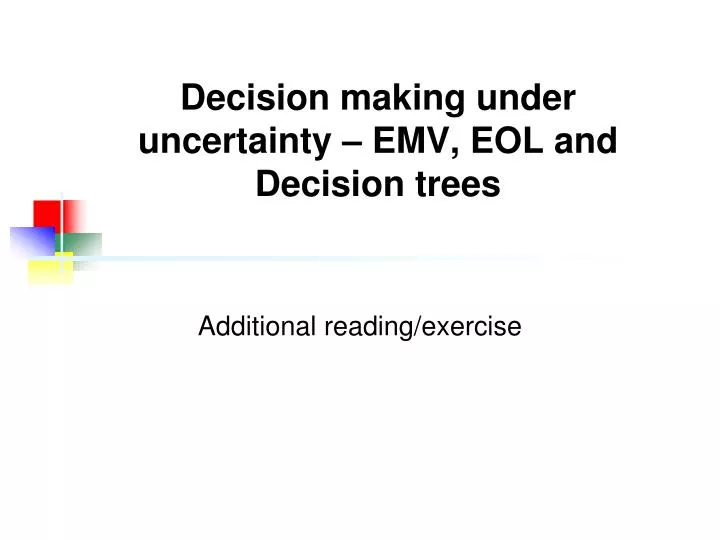
Decision making under uncertainty – EMV, EOL and Decision trees Additional reading/exercise
Steps involved in decision making under uncertainty • List alternative courses of action • Choices or actions • List uncertain events • Probability of occurrence of each action • Determine ‘payoffs’ • Associate a payoff with each event/outcome combination • Adopt decision criteria • Evaluate criteria for selecting the best course of action
List possible alternatives Two methods of showing alternatives unavailable under uncertain environments PayoffTable Decision Tree
Sample payoff table A payoff table shows alternatives, states of nature, and payoffs
Sample decision tree (graphical representation of payoff table) Strong Economy 200 Large factory Stable Economy 50 Weak Economy -120 Strong Economy 90 Average factory Stable Economy 120 Weak Economy -30 Strong Economy 40 Small factory Stable Economy 30 Weak Economy 20 Payoffs
Decision Criteria • Expected Monetary Value (EMV) • The expected profit for selecting an alternative • Expected Opportunity Loss (EOL) • The expected opportunity loss for selecting an alternative
EMV solution for the above example • The expected value is the weighted average payoff, given specified probabilities for each event Suppose these probabilities have been assessed for these three events
EMV solution for the above example Goal: Maximize expected value Example: EMV (Average factory) = 90(.3) + 120(.5) + (-30)(.2) = 81 Payoff Table: Maximize expected value by choosing Average factory Expected Values (EMV) 61 81 31
Expected Opportunity Loss Opportunity loss is the difference between an actual payoff for an action and the optimal payoff, given a particular event Payoff Table The action “Average factory” has payoff 90 for “Strong Economy”. Given “Strong Economy”, the choice of “Large factory” would have given a payoff of 200, or 110 higher. Opportunity loss = 110 for this cell.
Expected Opportunity Loss Payoff Table Opportunity Loss Table
EOL solution for the above example Goal: Minimize expected opportunity loss Example: EOL (Large factory) = 0(.3) + 70(.5) + (140)(.2) = 63 Opportunity Loss Table Minimize expected op. loss by choosing Average factory Expected Op. Loss (EOL) 63 43 93
Expected opportunity loss vs. expected monetary value • The Expected Monetary Value (EMV) and the Expected Opportunity Loss (EOL) criteria are equivalent. • Note that in this example the expected monetary value solution and the expected opportunity loss solution both led to the choice of the average size factory.
Decision tree analysis • A Decision tree shows a decision problem, beginning with the initial decision and ending will all possible outcomes and payoffs. Use a square to denote decision nodes Use a circle to denote uncertain events
Decision tree for the above example Strong Economy (.3) 200 Large factory Stable Economy (.5) 50 Weak Economy (.2) -120 (.3) Strong Economy 90 Average factory (.5) Stable Economy 120 (.2) Weak Economy -30 Decision (.3) Strong Economy 40 Small factory (.5) Stable Economy 30 (.2) Weak Economy 20 Uncertain Events Probabilities Payoffs
Calculate EMVs for each outcome node Strong Economy (.3) EMV=200(.3)+50(.5)+(-120)(.2)=61 200 Large factory Stable Economy (.5) 50 Weak Economy (.2) -120 (.3) Strong Economy EMV=90(.3)+120(.5)+(-30)(.2)=81 90 Average factory (.5) Stable Economy 120 (.2) Weak Economy -30 (.3) Strong Economy EMV=40(.3)+30(.5)+20(.2)=31 40 Small factory (.5) Stable Economy 30 (.2) Weak Economy 20
Make the decision Strong Economy (.3) EV=61 200 Large factory Stable Economy (.5) 50 Weak Economy (.2) -120 (.3) Strong Economy EV=81 90 Maximum EMV=81 Average factory (.5) Stable Economy 120 (.2) Weak Economy -30 (.3) Strong Economy EV=31 40 Small factory (.5) Stable Economy 30 (.2) Weak Economy 20