Download
1 / 35
350 likes | 357 Vues
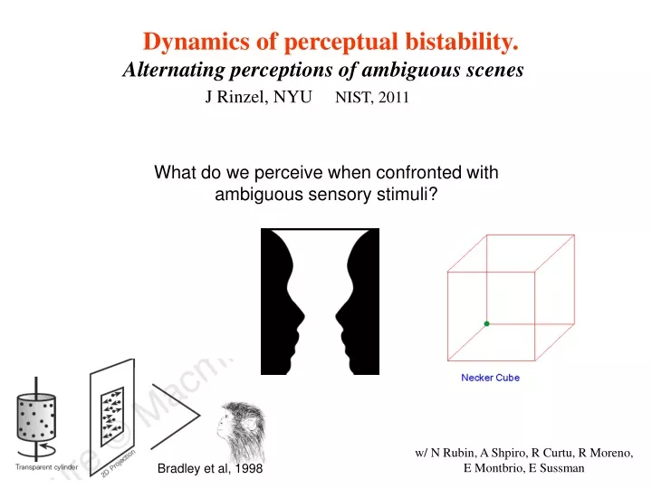
Bradley et al, 1998. Dynamics of perceptual bistability. Alternating perceptions of ambiguous scenes J Rinzel, NYU NIST, 2011. What do we perceive when confronted with ambiguous sensory stimuli?. w/ N Rubin, A Shpiro, R Curtu, R Moreno, E Montbrio, E Sussman.

E N D
Bradley et al, 1998 Dynamics of perceptual bistability. Alternating perceptions of ambiguous scenes J Rinzel, NYU NIST, 2011 What do we perceive when confronted with ambiguous sensory stimuli? w/ N Rubin, A Shpiro, R Curtu, R Moreno, E Montbrio, E Sussman
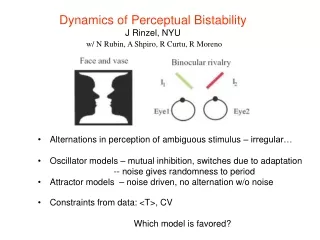
In binocular rivalry: present different images to each eye. Do we perceive an averaged image or…?
Dynamics of Perceptual Bistability • Visual modality: moving plaids; • Auditory modality: repeating triplet pattern • Neuronal-based models • Oscillator models -- • mutual inhibition + slow negative feedback (adaptation) • noise gives randomness to period • Attractor models – • noise driven, no alternation w/o noise • double-well potential: phenomenological model • Use stats to constrain models • Levelt II revisited: perceptual exploratory strategy • Auditory “objects” and alternations: ABA_ABA_… common principles. w/ N Rubin, A Shpiro, R Curtu, R Moreno, E Montbrio, E Sussman Funding: Swartz Foundation, NIH
PLAID DEMO R Moreno, N Rubin Transparent + coherent.Some parameter variations.
Triplet pattern (Van Noorden, 1975) -- possible ambiguityin auditory streaming. “galloping” Integration Sound parameters: DF = frequency difference PR = presentation rate Segregation Pressnitzer & Hupe, Current Biology, 2006
IV: Levelt, 1968 Mutual inhibition with slow adaptation alternating dominance and suppression
r1 r2 f Input, I1 I2 r1 r2 a2 Slow adaptation, a1(t) u τdr1/dt = -r1 + S(-βr2 - φ a1+ I1) τa da1/dt = -a1 + fa(r1) τ dr2/dt = -r2 + S(-βr1 - φ a2+ I2) τa da2/dt = -a2 + fa(r2) τa >> τ , S(u)=1/(1+exp[(θ-u)/k]) Oscillator Models for Directly Competing Populations Two mutually inhibitory populations, corresponding to each percept. Firing rate model: r1(t), r2(t) Slow negative feedback: adaptation or synaptic depression. S, fa r1 No recurrent excitation …half-center oscillator w/ N Rubin, A Shpiro, R Curtu Wilson 2003; Laing and Chow 2003 Shpiro et al, J Neurophys 2007
IV fa(u)=γu Alternating firing rates Adaptation slowly grows/decays Excessive symmetry adaptation LC model
Five Regimes of Behavior, Common to Neuronal Competition Models Shpiro et al, J Neurophys 2006 Curtu et al, SIADS, 2008 Increasing Stimulus depression LC model Wilson’s model
Math – adaptation model with adaptation dominant: φ > β / (1+τ). (I1=I2.) Dynamic states and stability depend on steepness of S and inhibition strength, β. Weak inhibition: SIM stable, for all I- no altern’ns Strong enough: then Hopf bifur’cns (2 of them) are supercritical and lead to anti-phase oscill’n. Very strong: multiple equilibria, pitchfork and, if stable, WTA. φ Five Regimes of Behavior, Common to Neuronal Competition Models Shpiro et al, J Neurophys 2006 Curtu et al, SIADS, 2008 φ depression LC model
Fast/Slow Dynamics r1- nullcline r2- nullcline r1 = S(- β r2 - φ a1+ I1) r2 = S(- β r1 - φ a2+ I2) r2 r1 Fast-Slow dissection: r1 , r2 fast variables a1 , a2 slow variables Decision making models, XJ Wang… a1, a2 frozen
Switching occurs when a1-a2 traj reaches a curve of SNs (knees) r2 a2 r1 a1 r1-r2 phase plane, slowly drifting nullclines • At a switch: • saddle-node in fast dynamics. • dominant r is high while system rides • near “threshold”of suppressed populn’s • nullcline ESCAPE. r1- nullcline r2- nullcline β =0.9, I1=I2=1.4
net input net input Small I, “release” input Large I, “escape” Dominant, a ↑ I – φ a I + α a – φ a θ θ Suppressed, a ↓ I – φ a - β Recurrent excitation, secures “escape” Switching due to adaptation: release or escape mechanism S rj = S(input to j) = S(- β rk - φ aj+ Ij) f
Noise leads to random dominance durations and eliminates WTA behavior. τdri/dt = -ri+ S(-βrj - φ ai+ Ii + ni) τa dai/dt = -ai + fa(ri) Added to stimulus I1,2 s.d., σ= 0.03, τn= 10 Model with synaptic depression
Noise-Driven Attractor Models w/ R Moreno, N Rubin J Neurophys 2007
Noise-Driven Attractor Models w/ R Moreno, N Rubin J Neurophys 2007 No oscillations if noise is absent. Kramers 1940 Noise-induced bursting. Sukbin Lim, NYU
LP-IV in an attractor model IV 2D model 1D model
WTA activity rA=rB OSC gA= gB Compare dynamical skeletons: “oscillator” and attractor-based models
Dynamical properties of a network with spiking neurons. Simulation results. Levelt II 100 LIF units/ popul’n distribution
Neuronal correlates of alternations Sheinberg and Logothetis, 1997 fMRI: Tong et al, 1998 fMRI: Polonsky et al, 2000 Electrophysiology: Leopold, Logothetis…
fMRI MEG From Sterzer et al, review, TICS, 2009 Rubin’s face-vase: early visual cortex. Parkkonen et al, PNAS, 2008
With noise 1 sec < mean T < 10 sec 0.4 < CV < 0.6 Noise-free Difficult to arrange high CV and high <T> in OSC regime. Observed variability and mean duration constrain the model.
With noise Favored: noise-driven attractor with weak adaptation – but not far from oscillator regime.
TA TB contrast B contrast B contrast A LP-II is not valid for all contrast values … LP-II in binocular rivalry Parameter dependence of mean T and f: 0.5 Eye B fraction B contrast A Eye A 0 0.14 contrast B ??? w/ Moreno, Shpiro, Rubin
Plaids with different wavelengths depth reversals Transparent + different frequencies.
Levelt’s II generalized, Moreno et al, J Vision (2010), ‘Parameter manipulation of an ambiguous stimulus affects mostly the mean dominance duration of the stronger percept.’ also Brascamp et al 2006 Alternation: a perceptual exploration strategy. Percent dominance reflects brain’s estimate of probability of depth. #1 behind #1 behind w/ Moreno, Shpiro, Rubin J of Vision, 2010
Maximum alternation rate at equidominance n=4 rivalry depth reversals plaids Moreno-Bote et al, J of Vision, 2010.
Models: Input normalization and maximum alternation rate at equidominance Alternation rate fraction of dominance w/ Moreno, Shpiro, Rubin
Temporal dynamics of auditory and visual bistability – common principles of perceptual organization. Pressnitzer & Hupe, 2006 Van Noorden, 1975
Visual Temporal dynamics of auditory and visual bistability – common principles of perceptual organization. Pressnitzer & Hupe, 2006 Integrated or segregated percepts Grouped or split percepts Exclusivity, randomness, and inevitability Leopold & Logothetis, 1999
Visual Temporal dynamics of auditory and visual bistability – common principles of perceptual organization. Pressnitzer & Hupe, 2006 Integrated or segregated percepts Grouped or split percepts Bistability/alternationin auditory streaming – integration (galloping) or segregation. 3 STs 4 STs Tone duration 120 ms, 3 STs, A=440 Hz, B=523 Hz
Visual Auditory Temporal dynamics of auditory and visual bistability – common principles of perceptual organization. Pressnitzer & Hupe, 2006 Integrated or segregated percepts Grouped or split percepts Exclusivity, randomness, and inevitability Leopold & Logothetis, 1999 w/ Montbrio
Direct demonstration of bistability for range of DF w/ Sussman, Montbrio ascend descend Tone duration 120ms, 4 reps
SUMMARY • Visual & auditory modality • Neuronal-based models • Oscillator models -- • mutual inhibition + slow negative feedback (adaptation) • noise gives randomness to period • Attractor models – • noise driven, no alternation w/o noise • double-well potential: phenomenological model • Use stats to constrain models • Levelt II revisited: perceptual exploratory strategy • Auditory “objects” and alternations: ABA_ABA_… common principles. w/ N Rubin, A Shpiro, R Curtu, R Moreno, E Montbrio, E Sussman Other works: Dayan ‘98, Lehky ‘88, Grossberg ’87, Wilson ‘01 Funding: Swartz Foundation, NIH
Schematic of bistability and hysteresis DF a1 adaptation a1 Some range of DF has bistability Range of a1for bistability Range of DF for bistability DF* #1 dominant & adapting DF = DF*, fixed #1 comes “on” r1 firing rate #1 goes “off” #1 suppressed & recovering from adaptation